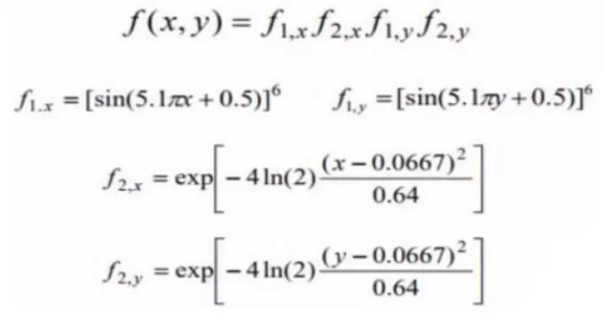
Week 4.1 - Genetic Algorithm

%% stalagmite_model_ with GA optimization challenge

clear all;
close all;
clc;

x = linspace(0,0.6,150);
y = linspace(0,0.6,150);
num_spaces = 30; % no of iterations

[xx, yy] = meshgrid(x , y); % creates a 2D mesh

for i = 1:length(xx)

    for j = 1:length(yy)
    
        input_vector(1) = xx(i,j);
        input_vector(2) = yy(i,j);
        f(i,j) = stalagmite(input_vector); % f(i,j) represent the elevation
    end
    
end

% % 1 Program for unbounded space
rng default % for reproducability
tic

for i = 1:num_spaces

    [input, Fval(i)] = ga(@stalagmite,2);
    xout(i) = input(1);
    yout(i) = input(2);
    
end
program1 = toc;

% Plotting unbounded space
figure(1)
subplot(2,1,1)
hold on
surfc(xx,yy,-f)
shading interp
plot3(xout,yout,-Fval,'marker', 'o')
subplot(2,1,2)
plot([1:30], -Fval)
xlabel('X range')
ylabel('Y range')
title('Unbounded inputs') % search space not defined in this version

% 2 Program for Bounded space

tic
lb = [0,0];
ub = [0.6,0.6];
rng default
for i = 1:num_spaces

    [input, Fval(i)] = ga(@stalagmite,2,[],[],[],[],lb,ub); % as there are no linear and non linear constraints to this function except for the bounds
    xout(i) = input(1);
    yout(i) = input(2);
    
end
program2 = toc;

% Plotting Program2
figure(2)
subplot(2,1,1)
hold on
surfc(x,y,-f)
shading interp
plot3(xout,yout, -Fval,'marker', 'o')
subplot(2,1,2)
plot(-Fval)
xlabel('X range')
ylabel('Y range')
title('Bounded inputs')

% 3 Program for bounded space with higher initial population size
options = optimoptions('ga','PopulationSize', 300);
tic

lb = [0,0];
ub = [0.6,0.6];
rng default
for i = 1:num_spaces

    [input, Fval(i)] = ga(@stalagmite,2,[],[],[],[],lb,ub,[],[],options);
    xout(i) = input(1);
    yout(i) = input(2);
    
end
program3 = toc;

% Plotting Program3
figure(3)
subplot(2,1,1)
hold on
surfc(x,y,-f)
shading interp
plot3(xout,yout, -Fval,'marker', 'o')
subplot(2,1,2)
plot(-Fval)
xlabel('X range')
ylabel('Y range')
title('Bounded inputs with higher Populationsize')

Below is the function to which stalagmite is to be applied

function [Outvar] = stalagmite(invar)


F_1x = sin(5.1*pi*invar(1)+0.5)^6;
F_1y = sin(5.1*pi*invar(2)+0.5)^6;

F_2x = exp(-4*log(2)*((invar(1)-0.0667)^2/0.64));
F_2y = exp(-4*log(2)*((invar(2)-0.0667)^2/0.64));

[Outvar] = -(F_1x*F_2x*F_1y*F_2y);

end

output:

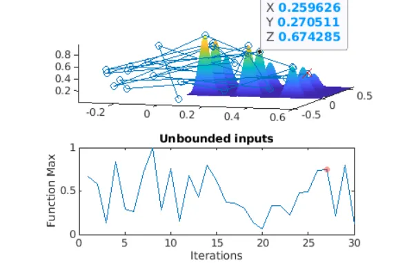
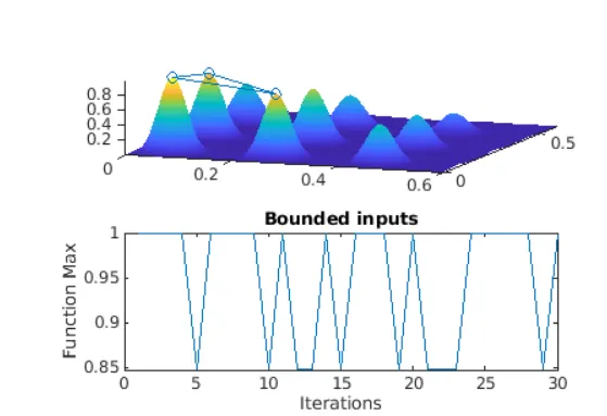
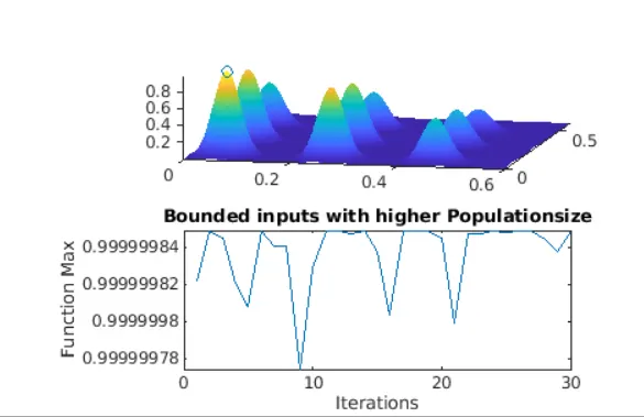
at x = 0.066, y = 0.066, the function is reaching global maxima of 1, as shown below: Here z represents the result from the stalagmite of the given function.

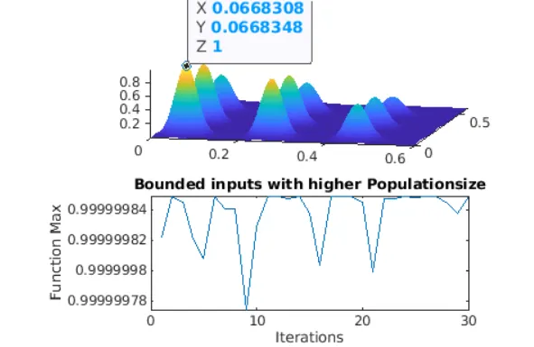
Stalagmite function purpose is to generate local maxima and minima, since these may vary from few to many. hence we use another mathematical algorithm inbuilt to Matlab, which is Ga to optimize the stalagmite function and generate a global maxima or minima. Usually GA function only generates global minima. We are rearranged the function so make the program display the global maxima instead.

This is optimization method is based on the sizing considered, time taken if recorded using different versions of the same program. Like shown above, three figures show the behavious of GA algorithm in unbounded search space, which usually takes less time and function output range is between 0 to 1, whereas second version is using a bounded space within a set x & y limits, and the output in 2nd version is ranging from 0.85 to 1 and finally, 3rd version is a refined program with more sizing thus giving more accuracy and sensitivity to the function.

The major difference in 2nd and 3rd version of the algorithm is that the time taken and also the output range, in case of 3rd version, the output is limiting to 1 and sensitivity level is to the power of 1e-6 to 1e^-7.

Lets now understand the ga algorithm and its applications:

GA are search based optimization algorithms inspired by the basic principles of biological evolution and natural selection.

Optimization is the process of finding the inputs which get the best output or a suitable output. meaning thereby whether maximizing or minimizing a certain function depending on our needs. The set of all possible values the inputs can take is called the search space, and a point lies in this search space which delivers us the optimal solution.

Ga used the concept of survival of the fittest to the functions subjected to any linear equalities or inequalities. In a pool of all possible solutions to any given problem and for each such solutions, will undergo crossovers, mutations to find more solutions and the process continuous, here the catch is more the pool size, more will be the combinations of solutions possible. Each solution will be assigned a fittness value based on this objective function value.

Thus the output off the GA gives us the inputs to the function to which optimization is needed, thus giving either maxima or minima. the pool size determines the sensitivity of the data. However the major drawback to this algorithm is that it uses random distribution of values to start with which is why in our 1st version, we see that solutions is offest to the region of our x & y limits.

Functions defined by non linear constraints, linear constraints and also function defined within a bounded region can be optimized using the GA function.

using options, we can increase the population size in order to get more combinations and better optimization. below shown message is because of the function tolerance in options, this is because the average fitness value generated for every best possible solution is less than the function tolerance given default in GA.

function used in this program for optimization is: