Week 3 - Solving second order ODEs

clear all
close all
clc
%% solving damped simple harmonic motion using second order ODE

% with base inputs like bob length, mass, g, damping coeff

% write a program to animate damped SHM as a function of time during the time interval 0-20sec and with initial conditions
% at time t=0, displacement = 0, angular displacement = 3 rad/sec

% ODE takes the form in this example as : d2theta/dt2 +(b/m)*dtheta/dt + (g/l)sin(theta) = 0
% from the above equation, we see that the resultant force on the system is zero and the system is a freely suspended bob attached to a string of length,l


% base inputs
b = 0.05 % damping coefficient N/m/s
g = 9.81 % m/sec2
m = 1 % kg
l = 1 %m
damp_status = 1; % 1 = on, 0 = OFF
Time_interval = linspace(0,20,1000);
theta = [0;3]; % initial boundary conditions, initial displacement and initial angular velocity
[t,soln] = ode45(@(t,theta) SHM_E1(t,theta,b,damp_status,g,l,m) , Time_interval, theta);

figure(1)
plot(t,soln(:,1),'r');
hold on
plot(t,soln(:,2 ),'k');
axis([0 20 -5 5])
grid on
legend('Angular displacement vs Time', 'Angular Velocity vs Time');
Time_period = 2*pi*(l/g)^0.5;
disp(num2str(Time_period,2));

position = soln(:,1);

for i=1:length(position)
   
   a = position(i); 
   x0=0;
   y0=0;
   
   x1 = l*sin(a);
   y1 = l*cos(a);
   
     %plotting the bob
   
   figure(2)
   plot(0,0,'o','markersize',4,'color','b','markerfacecolor','b');
   hold on
   plot([x0 x1],[y0 -y1],'linewidth',3,'color','b');
   plot([-2 2],[0 0],'linewidth',5,'color','g');
   hold on
   plot(x1,-y1,'o','markersize',12,'color','r','markerfacecolor','r');
   hold off
   axis([-2 2 -2 2]);
   grid on

   
end

Defining the function for second order ODE, and converting into first order ODE for the ODE45 to solve.

function dthetadt = SHM_E1(t,theta,b,Damp_status,g,l,m)

theta1 = theta(1);
theta2 = theta(2);

dthetadt1 = theta(2); % equation 1
dthetadt2 = -b/m*Damp_status*theta2-g/l*sin(theta1); % equation 2

dthetadt = [dthetadt1; dthetadt2];

end

A snapshot of the output is below:

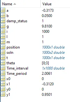
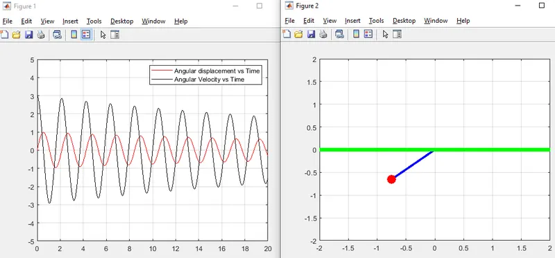
The Time period is also computed for this SHM, it is also observed that regardless of the damping effect the time period was maintained almost same observed every 10sec interval. Also the above SHM simulated a seconds pendulum of 0.5Hz.