Week 4.1 - Genetic Algorithm
Aim :
Write a program to optimize the stalagmite function and find its global maxima in MATLAB.
Objective :
- Understand the process of Optimization and its various types.
- Understand how the Genetic Algorithm works.
Introduction :
Optimization is the process of making something better.
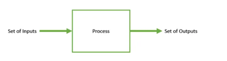
In any process, we have a set of inputs and a set of outputs. Optimization refers to finding the values of inputs in such a way that we get the best output. The definition of "best" in the mathematical term refers to maximizing or minimizing one or more objective functions by varying the input parameters. The set of all possible solutions which the input can take make up the search space. In this search space lies a set of points that give the optimal solution. The optimization process finds that set of points in the search space.
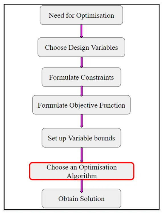
The following is the procedure followed by an optimization process.
Genetic algorithm :
As shown in the above flowchart, we need to choose an optimization algorithm to perform the. optimization process. Genetic Algorithm is one of the optimization processes. It is a search-based optimization technique based on the principles of genetics and natural selection. GA is frequently used to solve optimization problems in research and machine learning.
The GA process is as follows Step 1.. Determine the number of chromosomes, generation, and mutation rate and crossover
rate value
Step 2.. Generate chromosome-chromosome number of the population, and the initialization
value of the genes chromosome-chromosome with a random value Step 3.. Process steps 4-7 until the number of generations is met
Step 4.. Evaluation of fitness value of chromosomes by calculating objective function
Step 5.. Chromosomes selection
Step 6.. Crossover
Step 7.. Mutation
Step 8.. Solution (Best Chromosomes)
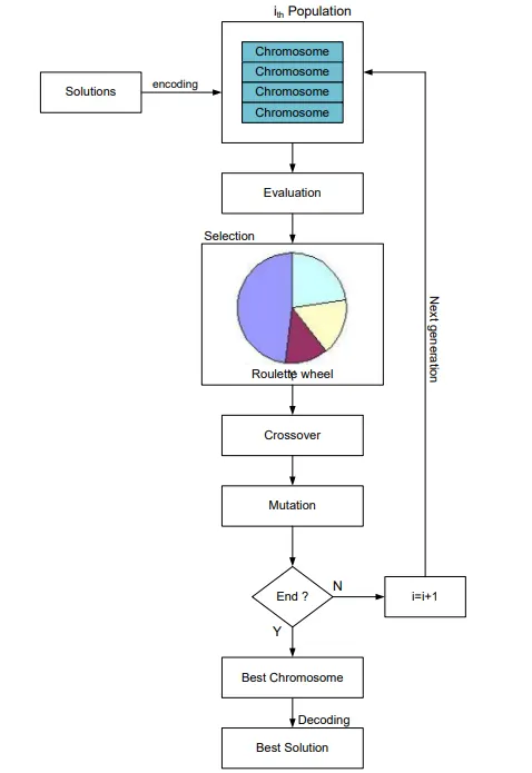
Genetic Algorithm uses three main types of rules at each step to create the next generation from the current population.
Selection rules : Select the individuals, called parents, that contribute to the popution at the next generation.
Crossover rules : Combine parentsto form children for the next generation.
Mutation rules : Apply random changes to individual parentsto form the children.
FITNESS FUNCTION -- The fitness function takes the solution as input and produces the suitability as the output. This evaluates how close the solution is to the optimal solution of the desired problem.
Syntax for GA : x = ga(fun,nvars,A,B,Aeq,Beq,lb,ub,nonlcon,Intcon,options)
where
x - variable to store output of the GA
fun - function handle to call the function
A,B - used to represent the linear inequalities of the function
Aeq,Beq - used to represent equality constraints
lb,ub - used to specify the lower and upper bounds of the variables of the function
nonlcon - represents non-linear constraints
Intcon - represents the integer constraint, such that the value of the function is an integer
options - used to provide the value of the default parameters; done using optimoptions
STALAGMITE FUNCTION :
A stalagmite is a type of rock formation that rises from the floor of a cave due to the accumulation of material deposited on the floor from ceiling drippings.
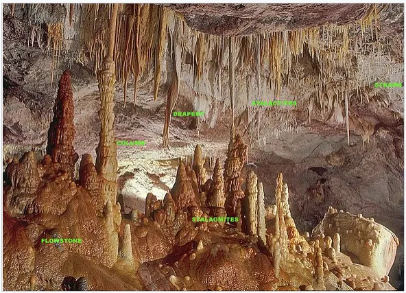
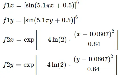
The following is the given stalagmite function for which we need to find the global maxima.
f(x,y) = f1x.f2x.f1y.f2y
where
MATLAB program :
FUNCTIOn
function [Fxy] = stalagmite(input_vector)
x = input_vector(1);
y = input_vector(2);

% Genetic Algorithm for a stalgamite function to find its minima
f1x = (sin(5.1*pi*x + 0.5))^6;
f2x = exp(-4*log(2)*((x-0.0667)^2)/(0.64));
f1y = (sin(5.1*pi*y + 0.5))^6;
f2y = exp(-4*log(2)*((y-0.0667)^2)/(0.64));

Fxy =  -(f1x*f2x*f1y*f2y);  % "-" is ued to invert the plot
end
MAIN PROGRAM
clear all
close all
clc
%%%% To study the statistical behavior of GA %%%%

% Create one-dimensional array x, y
% Define our search space
x = linspace(0, 0.6, 150);
y = linspace(0, 0.6, 150);
%Create two-dimensional array xx, yy
[xx, yy] = meshgrid(x,y);

num_cases = 50;  % run the GA 50 times

%%% Evaluating the stalagmite function
% For each value of x and y, create an array 'input vector'
for i = 1:length(xx)
    for j = 1:length(yy)
        input_vector(1) = xx(i,j);
        input_vector(2) = yy(i,j);
        f(i,j) = stalagmite(input_vector);
    end
end

%% Study 1 -- Statistical behavior

%tic and toc commands used to measure how long it takes to complete a study
tic

for i = 1 : num_cases
    [inputs, fopt(i)] = ga(@stalagmite,2); % calling the GA & passing no. of variables as inputs = 2
   % storing x and y values & and also the optimum value the function predicts
    xopt(i) = inputs(1);
    yopt(i) = inputs(2);
end
Study1_time = toc
figure(1)
subplot(2,1,1)   % Multiple subplots in the same figure window
hold on
surfc(x,y,f)   % first plot ---- a surface
shading interp
% plot x, y & the optimum func. value that GA predicts out of 50 studies
plot3(xopt, yopt, fopt, 'marker', 'o', 'markersize', 5, 'markerfacecolor', 'r')
title('Unbounded inputs')
subplot(2,1,2)   % second subplot to plot fopt
plot(fopt)
xlabel('Iterations')
ylabel('Function minimum')


%% Study2 -- Statistical behavior with upper and lower bounds
tic
for i = 1:num_cases
    [inputs, fopt(i)] = ga(@stalagmite,2,[],[],[],[],[0;0],[1;1]);   %GA syntax
    xopt(i) = inputs(1);
    yopt(i) = inputs(2);
end
study2_time = toc

figure(2)
subplot(2,1,1)
hold on
surfc(x,y,f)
shading interp
plot3(xopt, yopt, fopt, 'marker', 'o', 'markersize', 5, 'markerfacecolor', 'r')
title('Bounded inputs')
subplot(2,1,2)
plot(fopt)
xlabel('Iterations')
ylabel('Function minimum')


%% Study3 -- Increasing GA iterations
options = optimoptions('ga');
options = optimoptions(options, 'Populationsize', 170);

tic
for i = 1:num_cases
     [inputs, fopt(i)] = ga(@stalagmite,2,[],[],[],[],[0;0],[1;1],[],[],options);
    xopt(i) = inputs(1);
    yopt(i) = inputs(2);
end
study3_time = toc;

figure(3)
subplot(2,1,1)
hold on
surfc(x,y,f)
shading interp
plot3(xopt, yopt, fopt, 'marker', 'o', 'markersize', 5, 'markerfacecolor', 'r')
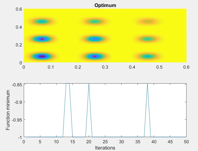
title('Optimum')
subplot(2,1,2)
plot(fopt)
xlabel('Iterations')
ylabel('Function minimum')
Output :
ITERATION_1
Study1_time =
6.0550
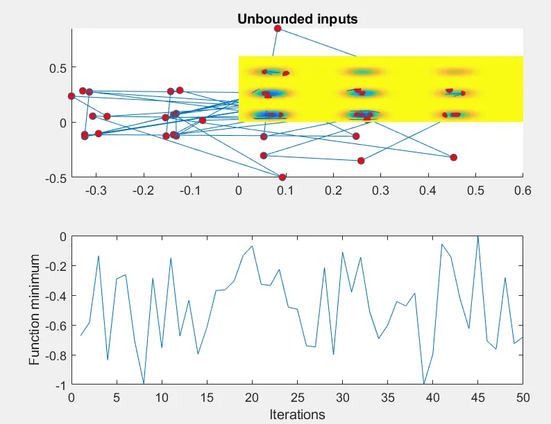
ITERATION_2
study2_time =
9.3626
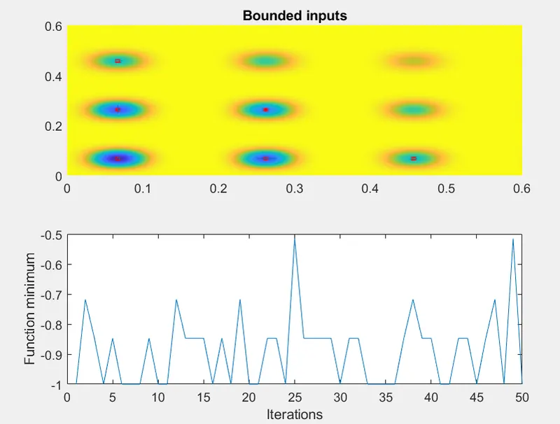
ITERATION_3