Week 3 - Solving second order ODEs

Aim :

Write a program to simulate the motion of a simple pendulum with damping in MATLAB.

Objective :

• Understand the transient behavior of a system.
• To be able to solve any Ordinary differential equation (ODE).

Introduction :

ODE is used to describe the transient behavior of a system. A simple example is a pendulum. The way the pendulum moves depends on Newton's second law. When this law is written down, we get a second-order Ordinary Differential Equation that describes the position of the ball with respect to time.

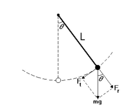
The figure shows a pendulum, with a string of zero mass and length 'L' and a bob of mass 'M'. When the bob is moved from its rest position and let go, it swings back and forth. The time it takes the pendulum to swing back and forth once is the period of the pendulum. The primary forces acting on the bob are i)Gravitational force and ii)Damping force from friction at the pivot and air resistance.

Let s(t) be the distance along the arc from the lowest point to the position of the bob at time 't', with displacement to the right considered positive. The figure shows tangential and radial components of the positive. Let theta(t) be the corresponding angle with respect to the vertical.

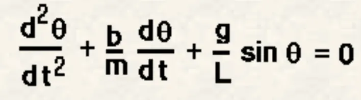
In the above equation,

g = gravity in m/s2,

L = length of the pendulum in m,

m = mass of the ball in kg,

b=damping coefficient.

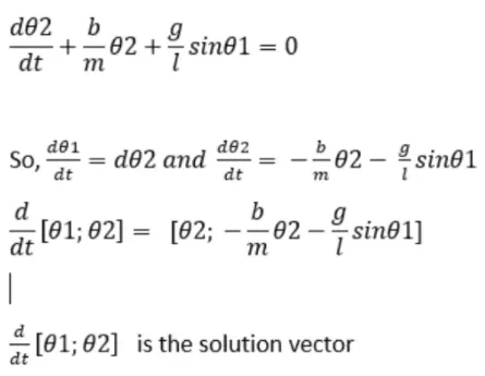
From the equation, let θ = θ1 and dθ/dt = dθ1/dt = θ2 --------- eq(1)

----------- eq(2)

Matlab program :

Function

function [dTheta_dt] = ode_func(t,Theta,b,g,l,m)
Theta1 = Theta(1)
Theta2 = Theta(2)
dTheta1_dt = Theta2;
dTheta2_dt = (-b/m)*Theta2 - (g/l)*sin(Theta1);
dTheta_dt = [dTheta1_dt;dTheta2_dt];
end

Program to simulate a pendulum having simple harmonic motion

clear all
close all
clc

b = 0.05;  % Damping coefficient
g = 9.81;  % acceleration of Gravity  (m/(s^2))
l = 1;  % Length of the string  (m)
m = 0.1;  % mass  (kg)

%%% Initial condition %%%
%Initial angular Displacement = 0
%Initial angular Velocity = 5 rad/s
Theta_0 = [0;5];

%%% Time points %%%
% Integrating ODE system to obtain solution
% Time between 0 to 20 seconds with 500 values in between
t_span = linspace(0,20,500);

%%% Solve ODE %%%
% ode45(@(t,Theta) --> define ODE as a function of t and Theta
% ode_func(___) --> how our ODE function is defined
[t, results] = ode45(@(t,Theta) ode_func(t,Theta,b,g,l,m),t_span,Theta_0);

%%% Plot %%%
figure(1)
plot(t,results(:,1))
hold on
plot(t,results(:,2))
ylabel('Plot')
xlabel('Time[s]')
title('Damped harmonic motion of a pendulum')
legend('Angular Dispacement','Angular Velocity')

%%% for loop %%%
ct = 1;
for i = 1:length(results(:,1))
% Initial position of the pendulum
x_start = 0
y_start = 0
% Final position of the pendulum    
x_end = l*sin(results(i,1))
y_end = -l*cos(results(i,1))

figure(2)
% Base
plot([-0.1,0.1],[0,0],'linewidth',5)
hold on;
% Pendulum string
line([x_start x_end],[y_start y_end],'linewidth',3)
hold on;
% Pendulum ball
plot(x_end,y_end, 'o','markers',30)
axis([-2 2 -2 2])
pause(0.01)
hold off;
M(ct) = getframe(gcf);
ct = ct+1
end

movie(M)
videofile = VideoWriter('Damping_Motion_of_Pendulum.avi','Uncompressed AVI');
open(videofile)
writeVideo(videofile,M)
close(videofile)

Output :

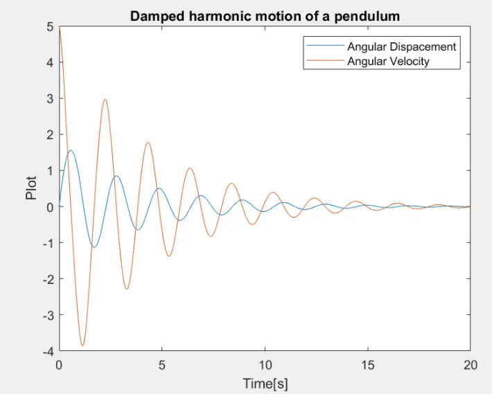
Video: Link for the Video of the animation of the motion of the pendulum.

https://youtu.be/j8C-KspfA0A