Week 4.1 - Genetic Algorithm
AIM : To write a code in MATLAB to optimise the stalagmite function and find the global maxima of the function.
OBJECTIVES :
- Write a code in MATLAB to optimise the stalagmite function and find the global maxima of the function.
- Clearly expalin the concept of genetic algorithm in your own words and also explain the syntax for ga in MATLAB in your report.
- Plot graphs for all 3 studies and for F maximum vs no. of iterations. Title and axes labels are a must.
INTRODUCTION :
A Genetic Algorithm is a strategy that guide us to solve both constrained and unconstrained optimization problems based on Charle's Darwin theory of natural selection. This algorithm reproduces the process of natural selection where the appropriate individual are selected for reproduction in order to produce offspring of next generation.
Genetic algorithms are commonly used to generate high-quality solutions to optimization and search problems by relying on biologically inspired operators such as mutation, crossover and selection.
Five phases are considered in a genetic algorithm.
- Initial population
- Fitness function
- Selection
- Crossover
- Mutation
Initial population
The process begins with a set of individuals which is called a Population. Each individual is a solution to the problem you want to solve.
An individual is characterized by a set of parameters (variables) known as Genes. Genes are joined into a string to form a Chromosome (solution).
In a genetic algorithm, the set of genes of an individual is represented using a string, in terms of an alphabet. Usually, binary values are used (string of 1s and 0s). We say that we encode the genes in a chromosome.
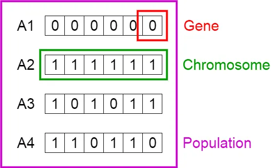
Population,Chromosomes and Genes
Fitness Function
The fitness function determines how fit an individual is (the ability of an individual to compete with other individuals). It gives a fitness score to each individual. The probability that an individual will be selected for reproduction is based on its fitness score.
Selection
The idea of selection phase is to select the fittest individuals and let them pass their genes to the next generation.
Two pairs of individuals (parents) are selected based on their fitness scores. Individuals with high fitness have more chance to be selected for reproduction.
Crossover
Crossover is the most significant phase in a genetic algorithm. For each pair of parents to be mated, a crossover point is chosen at random from within the genes.
For example, consider the crossover point to be 3 as shown below.
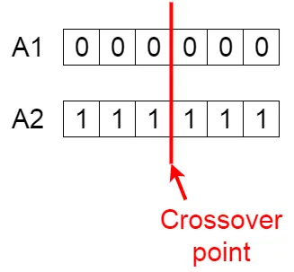
Crossover Point
Offspring are created by exchanging the genes of parents among themselves until the crossover point is reached.
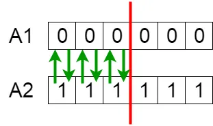
Exchanging genes among parents
The new offspring are added to the population.
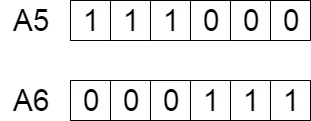
New Offspring
Mutation
In certain new offspring formed, some of their genes can be subjected to a mutation with a low random probability. This implies that some of the bits in the bit string can be flipped.
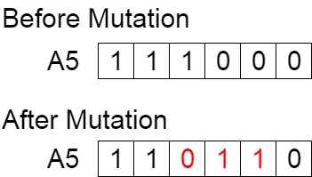
Mutation : Before and After
Mutation occurs to maintain diversity within the population and prevent premature convergence.
SYNTAX FOR GA :
x = ga( finds a local unconstrained minimum, fun,nvars)x, to the objective function, fun. nvars is the dimension (number of design variables) of fun.
x = ga( subjects the minimization to the constraints defined in fun,nvars,A,b,Aeq,beq,lb,ub,nonlcon)nonlcon. The function nonlcon accepts x and returns vectors C and Ceq, representing the nonlinear inequalities and equalities respectively. ga minimizes the fun such that C(x) ≤ 0 and Ceq(x) = 0. (Set lb=[] and ub=[] if no bounds exist.)
x = ga( minimizes with the default optimization parameters replaced by values in fun,nvars,A,b,Aeq,beq,lb,ub,nonlcon,options)options. (Set nonlcon=[] if no nonlinear constraints exist.) Create options using optimoptions.
x = optimum solution
f = ga(fun,nvars,A,b,[],[],lb,ub,nonlcon,Intcon,options)
fun = fitness function
nvars = number of variables
A,b = Linear inequality constraints
Aeq,beq = Linear equality constraints
lb = lower bound limit
ub = upper bound limit
nonlcon = Use of nonlinear constraint
Intcon = to get solution in integer
Options = To set population size minimize with non-default options.
STEPS INVOLVED IN GA STALAGMITE CODING :
- Stalagmite equation for genetic algorithm
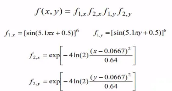
- Another step is converting these equation in function in MATLAB for GA solving
- To find global maxima we have to invert the equations, so to do that just multiply with [-1]
f = -(f1*f2*f3*f4)
CODING FITNESS FUNCTION :
The main thing while writing the function code is that we have to save the function in the same name of the function, For here it is "stalagmite.m"
% Equation input

 function A = stalagmite(input_vector)
            x = input_vector(1);
            y = input_vector(2);

            f1 = (sin(5.1*pi*x+0.5)).^6;
            f2 = exp((-4*log(2)*((x-0.0667).^2))/0.64);
            f3 = (sin(5.1*pi*y+0.5)).^6;
            f4 = exp((-4*log(2)*((y-0.0667).^2))/0.64);

 A = -(f1*f2*f3*f4);

end- The above stalagmite equation for GA is coded in stalagmite.m having 2 variables x&y.
- These function will be called in the program.
GET_STALAGMITE CODE :
function[f] = get_stalagmite(x,y)

% Creating a 2Dimensional mesh
[xx yy] = meshgrid(x,y);

% Evaluating the stalagmite function
for i = 1:length(xx)
    for j = 1:length(yy)
        input_vector(1) = xx(i,j);
        input_vector(2) = yy(i,j);
        f(i,j) = stalagmite(input_vector);
    end
end- For creating 2D mesh we will write a meshgrid between particular two coordinates & for code, it will be x,y
- Evaluating the stalagmite function using for loop and we called the main funtion which is stored in name of stalagmite.m
MAIN CODE :
clear all
close all
clc

% Inputs
x = linspace(0,0.6,150);
y = linspace(0,0.6,150);
num_cases = 50
f = get_stalagmite(x,y);

tic
% Study1 - Unbounded statistical behavior
for i = 1:num_cases
    [inputs,fopt(i)] = ga(@stalagmite,2);
    xopt(i) = inputs(1);
    yopt(i) = inputs(2);
end
study1_time = toc

% Plotting
figure(1)
subplot(2,1,1)
hold on
surfc(x,y,-f)
shading interp
xlabel('x value')
ylabel('y value')
plot3(xopt,yopt,-fopt,'marker','o','markersize',5,'markerfacecolor','r')
title('Unbounded inputs')
subplot(2,1,2)
plot(-fopt)
xlabel('Iterations')
ylabel('Function maximum')

tic
% Study2 - Statistical behavior with lower and upper bound
for i = 1:num_cases
    [inputs,fopt(i)] = ga(@stalagmite,2,[],[],[],[],[0;0],[1;1]);
    xopt(i) = inputs(1);
    yopt(i) = inputs(2);
end

study2_time = toc

figure(2)
subplot(2,1,1)
hold on
surfc(x,y,-f)
shading interp
xlabel('x value')
ylabel('y value')
plot3(xopt,yopt,-fopt,'marker','o','markersize',5,'markerfacecolor','r')
title('Bounded inputs')
subplot(2,1,2)
plot(-fopt)
xlabel('Iterations')
ylabel('Function maximum')

% Study3 - Increasing GA iterations
options = optimoptions('ga')
options = optimoptions(options,'populationsize',250);

tic
for i = 1:num_cases
    [inputs,fopt(i)] = ga(@stalagmite,2,[],[],[],[],[0;0],[1;1],[],[],options);
    xopt(i) = inputs(1);
    yopt(i) = inputs(2);
end

study3_time = toc

figure(3)
subplot(2,1,1)
hold on
surfc(x,y,-f)
shading interp
xlabel('x value')
ylabel('y value')
plot3(xopt,yopt,-fopt,'marker','o','markersize',5,'markerfacecolor','r')
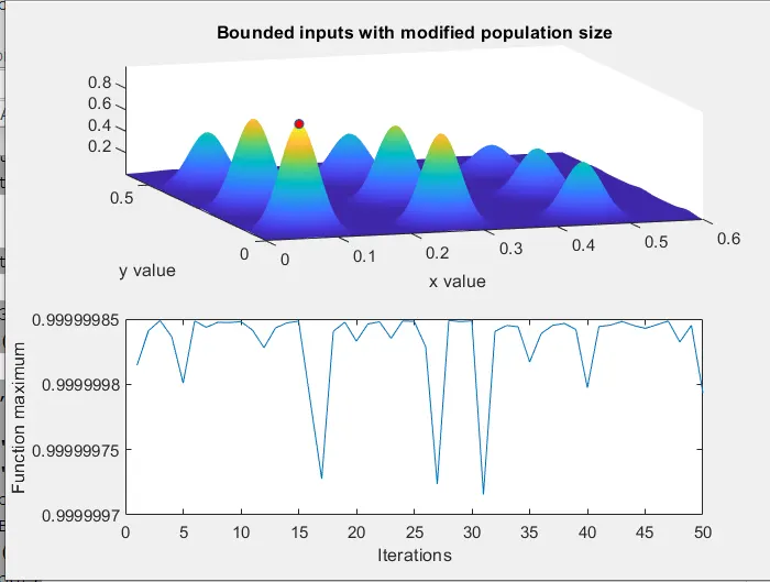
title('Bounded inputs with modified population size')
subplot(2,1,2)
plot(-fopt)
xlabel('Iterations')
ylabel('Function maximum')
- Firstly, clear all, close all &clc command were used to clear workspace close all figures and erased all other.
- The search space of ga is define using linspace command the variable lies between 0 to 0.6 with 150 values in between.
- The number of cases means these were the iterations i.e. ga will run for 50 times.
- The get_stalagmite.m function was called
- For loop was used to give inputs to get_stalagmite function inputs which means while running 50 iterations the value changes.
- We had executed 3 different studies ; 1. Unbounded statistical behavior; 2. Bounded statistical behavior; 3. Bounded with increase population size.
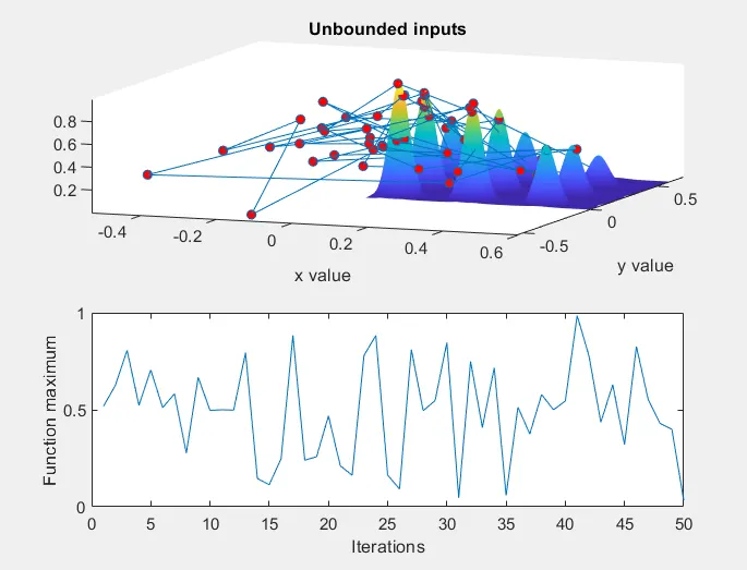
- Study1 :- In this the optimum values for inputs taken for each iterations with the help of a for loop.
- Study timers commands tic & toc are used to record the study time.
- The 'ga' syntax used in first study (Unbounded statistical behavior) ; X = ga(fun,nvars)
- Plotting commands : Figure command is used for opening a figure window and subplot command is used to get multiple plot in one figure window.
- Now for creating a 2D surface for stalagmite, we have to write "surfc(x,y,f)"
- Proper shading the surface we have to write a code for that and that will be "shading interp". If we will not provide shading then it will create mesh structure on stalagmite.
- plot3 command was used for getting surface as 3D
- Then the title command is used for getting title for plot and label the plot.
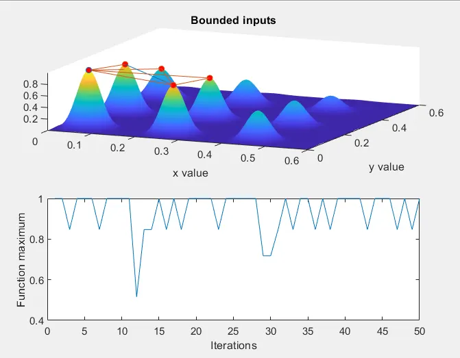
- Study2 :- Sa,e parameters were used only difference is in using the syntax of 'ga', x = ga(fun,nvars,A,b,Aeq,beq,lb,ub) i.e. using lower and upper bound limit.
- Study3 :- The plotting and other command were as same as above but syntax for ga changed by using optimoptions and increades iterations/populationsize is 250.
- The 'ga' syntax for 3rd study is : x = ga(fun,nvars,A,b,Aeq,beq,lb,ub,nonlcon,Intcon,options)
STUDY TIME :
- study1_time = 2.4117
- study2_time = 5.3328
- study3_time = 9.6320
OUTPUTS OBTAINED :
Output of Study1 :
Output of Study2:
Output of Study3 :
CONCLUSION :
- There were different types of syntax used for diffrent equations.
- The perfect global maxima can be obtained by increasing the population size.
- The 'ga' is used to find minimum value for maximum value we need to inverse it that's why we multiply formula by [-1] in stalagmite.m
- The study time increases with respect to population size.
REFERENCES :
https://en.wikipedia.org/wiki/Genetic_algorithm
https://in.mathworks.com/help/gads/what-is-the-genetic-algorithm.html
https://in.mathworks.com/help/gads/what-is-the-genetic-algorithm.html