Week 3 - Solving second order ODEs

AIM : To write a program that solves the following ODE. This ODE represents the equation of motion of a simple pendulum with damping.

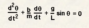
In the above equation,

g = gravity in m/s2,

L = length of the pendulum in m,

m = mass of the ball in kg,

b=damping coefficient.

Simulate the motion between 0-20 sec, for angular displacement=0,angular velocity=3 rad/sec at time t=0.

INTRODUCTION :

• Pendulum, body suspended from a fixed point so that it can swing back and forth under the influence of gravity. Pendulums are used to regulate the movement of clocks because the interval of time for each complete oscillation, called the period, is constant. The formula for the period T of a pendulum is T = 2π Square root of√^L/_g, where L is the length of the pendulum and g is the acceleration due to gravity.

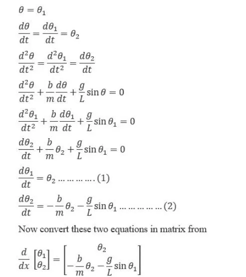
For solving ODE USING MATLAB, higher order differential equation need to convert into set of single order differential equation.

Parameters taken for study are as follows:

L=1 metre,

m=1 kg,

b=0.05.

g=9.81 m/s2.

Simulate the motion between 0-20 sec, for angular displacement=0,angular velocity=3 rad/sec at time t=0.

FUNCTION CODE :

function [dtheta_dt] = ode_function(t,theta,b,g,l,m)
         theta1 = theta(1)
         theta2 = theta(2)
         dtheta1_dt = theta2
         dtheta2_dt = -(b/m)*theta2-(g/l)*sin(theta1);
         dtheta_dt = [dtheta1_dt;dtheta2_dt];
end

Ode_function converts second order differential equation into single order using time limits and theta values.

MAIN PROGRAM :

clear all 
close all
clc

b = 0.05;
g = 9.87;
l = 1;
m = 0.1;
%Initial Conditions
theta = [0;3];

% Time points 
t_span = linspace(0,20,500);

% Solve ODE
[t,results] = ode45(@(t,theta)ode_function(t,theta,b,g,l,m),t_span,theta)
plot(t,results(:,1))
hold on 
plot(t,results(:,2))
ylabel('plot')
xlabel('time')
legend('displacement','velocity')
title('Displacement & Velocity graph')

%Creating motion of pendulum
ct = 1 


for i = 1:length(t)
    X0 = 0
    Y0 = 0
    
    X1 = l*sin(results(i,1));
    Y1 = -l*cos(results(i,1));
    
    figure(2)
    plot([X0,X1],[Y0,Y1],'linewidth',5,'color','g')
    hold on
    plot(X1,Y1,'o','markersize',20,'markerfacecolor','r')
    
    plot([-1 1],[0 0],'linewidth',5,'color','b')
    axis([-2 2 -2 2])
    title('Motion of Pendulum')
    xlabel('X')
    ylabel('Y')
    pause(0.03)
    hold off
    M(ct) = getframe(gcf);
    ct = ct+1;
    
end

%Create Movie
movie(M)
Videofile = VideoWriter('ode_simple_pendulum.avi','Uncompressed AVI');
open(Videofile)
writeVideo(Videofile,M)
close(Videofile)

EXPLAINATION :

1. clear all :- Removes data from workspace.
2. close all :- Delete the current figure.
3. clc :- clear all input and output from command window.
4. Define the input parameters to the ODE i.e. damping coefficient, gravity, mass of pendulum and length of pendulum.
5. Assign the input conditions given, diplacement = 0 & velocity = 3rad/s and time limits to integrate the equation.
6. For solving ODE we need to call the function ode_function and assign the parameters.
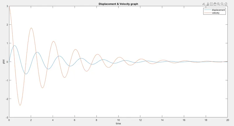
7. Plot the results for desplacement and velocity using plot command.Label the axis and give title to graph using title command. legend command was used to specify which is curve for displacement & velocity.
8. For creating motion of pendulum, firstly, we defined the co-ordinates of pendulum i.e. X0,Y0,X1 & Y1 using trignometric relations.
9. Plot the co-ordinates of pendulum. And define the axis for the pendulum using axis command. Give the title and label the axis. 'M' was used to create movie.
10. Creating movie by connecting all the frames, define video format using VideoWriter then open video, write video and after that close the video.

GRAPH OF DISPLACEMENT & VELOCITY :

ANIMATION OF SIMPLE PENDULUM :

https://youtu.be/nmalEiKXYlI