Week 4.1 - Genetic Algorithm
Week 4- Genetic Algorthim
- Objective:
- Write a code in MATLAB to optimize the stalagmite function and find the global maxima of the function.
- Clearly expalin the concept of genetic algorithm in your own words and also explain the syntax for ga in MATLAB in your report.
- Make sure that your code gives the same output, even if it is made to run several times.
- Plot graphs for all 3 studies and for F maximum vs no. of iterations. Title and axes labels are a must, legends could be shown if necessary.
What’s meant by global optimization?
Optimization refers to finding the set of inputs to an objective function that results in the maximum or minimum output from the objective function.
It is common to describe optimization problems in terms of local vs. global optimization.
Local vs. Global Optima
Optimization is the process of finding the point that minimizes a function. More specifically:
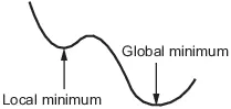
- A local minimum of a function is a point where the function value is smaller than or equal to the value at nearby points, but possibly greater than at a distant point.
- A global minimum is a point where the function value is smaller than or equal to the value at all other feasible points.
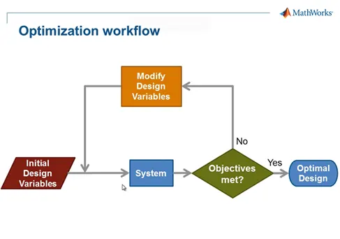
Optimization workflow.
What is meant by genetic algorithm ?
Genetic algorithms are inspired by Darwin's theory of evolution. Solution to a problem solved by genetic algorithms uses an evolutionary process (it is evolved).
Algorithm begins with a set of solutions (represented by chromosomes) called population. Solutions from one population are taken and used to form a new population. This is motivated by a hope, that the new population will be better than the old one. Solutions which are then selected to form new solutions (offspring) are selected according to their fitness - the more suitable they are the more chances they have to reproduce.
This is repeated until some condition (for example number of populations or improvement of the best solution) is satisfied.
Genetic Algorithms(GAs) are adaptive heuristic search algorithms that belong to the larger part of evolutionary algorithms. Genetic algorithms are based on the ideas of natural selection and genetics. These are intelligent exploitation of random search provided with historical data to direct the search into the region of better performance in solution space. They are commonly used to generate high-quality solutions for optimization problems and search problems.
Genetic algorithms simulate the process of natural selection which means those species who can adapt to changes in their environment are able to survive and reproduce and go to next generation. In simple words, they simulate “survival of the fittest” among individual of consecutive generation for solving a problem. Each generation consist of a population of individuals and each individual represents a point in search space and possible solution. Each individual is represented as a string of character/integer/float/bits. This string is analogous to the Chromosome.
Foundation of Genetic Algorithms
Genetic algorithms are based on an analogy with genetic structure and behavior of chromosome of the population. Following is the foundation of GAs based on this analogy –
- Individual in population compete for resources and mate
- Those individuals who are successful (fittest) then mate to create more offspring than others
- Genes from “fittest” parent propagate throughout the generation, that is sometimes parents create offspring which is better than either parent.
- Thus each successive generation is more suited for their environment.
- Operators of Genetic Algorithms
- Once the initial generation is created, the algorithm evolve the generation using following operators –
1) Selection Operator:The idea is to give preference to the individuals with good fitness scores and allow them to pass there genes to the successive generations.
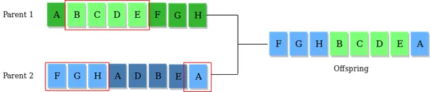
2) Crossover Operator: This represents mating between individuals. Two individuals are selected using selection operator and crossover sites are chosen randomly. Then the genes at these crossover sites are exchanged thus creating a completely new individual (offspring). For example –
Mutation Operator: The key idea is to insert random genes in offspring to maintain the diversity in population to avoid the premature convergence. For example –
The whole algorithm can be summarized as –
1) Randomly initialize populations p
2) Determine fitness of population
3) Until convergence repeat:
a) Select parents from populatio
b) Crossover and generate new populatio
c) Perform mutation on new population
Stalagmite function:
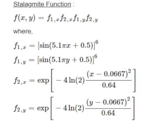
Stalagmite function code;
%stalagmite Function

function[stalagmite] = stalagmite(input_vector)

x = input_vector(1);
y = input_vector(2);
f1x = (sin((5.1*pi*x)+0.5))^6;  %the first term
f1y = (sin((5.1*pi*y)+0.5))^6;  %the second term
f2x = exp((-4*log(2)*(x-0.0667)^2)/0.64);  %the 3rd term
f2y = exp((-4*log(2)*(y-0.0667)^2)/0.64);  %the 4th term

stalagmite = -(f1x*f1y*f2x*f2y);

end
Main code
%case 1
% progrman to find global maxima using genetic algorthim

clear all
close all
clc
%1D Array _defining our search space
x = linspace(0,0.6,150);
y = linspace(0,0.6,150);
  num_cases = 50;

 %creating 2D array using meshgrid funciton

 [xx yy] = meshgrid(x,y);

 % study case no:1 Unbound inputs
for i = 1:length(xx)
    for j = 1:length(yy)
        input_vector(1) = xx(i,j);
        input_vector(2) = yy(i,j);
        f(i,j) = stalagmite(input_vector);

    end
end
%iterations of genetic algorthim
tic
for i = 1:num_cases
    [inputs, fopt(i)] = ga(@stalagmite,2);
    xopt(i) = inputs(1);
    yopt(i) = inputs(2);
end

study1_time = toc

figure (1)
subplot(2,1,1)
hold on
surfc(xx,yy,-f)
shading interp
title('Unbounded Inputs')
plot3(xopt,yopt,-fopt,'marker',5,'markerfacecolor','r')
xlabel('x axis')
ylabel('y axis')
zlabel('f(x,y)')
subplot(2,1,2)
plot(-fopt)
xlabel('Iterations')
ylabel('Global Maxima')
title('Global Maxima vs Iterations')
axis([0 50 0 1.5])
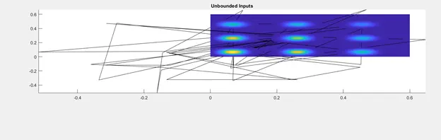
Results;
time taken: 6.3989 seconds
Porgram code of case_2;
%case 2
% progrman to find global maxima using genetic algorthim

clear all
close all
clc
%1D Array _defining our search space
x = linspace(0,0.6,150);
y = linspace(0,0.6,150);
  num_cases = 50;

 %creating 2D array using meshgrid funciton

 [xx yy] = meshgrid(x,y);

 % study case no:1 Unbound inputs
for i = 1:length(xx)
    for j = 1:length(yy)
        input_vector(1) = xx(i,j);
        input_vector(2) = yy(i,j);
        f(i,j) = stalagmite(input_vector);

    end
end
%iterations of genetic algorthim

%defining population size

options = optimoptions('ga')
options = optimoptions(options,'PopulationSize',250)
tic
for i = 1:num_cases
    [inputs, fopt(i)] = ga(@stalagmite,2,[],[],[],[],[0;0],[0.6;0.6]); %bound inputs
    xopt(i) = inputs(1);
    yopt(i) = inputs(2);
end

study2_time = toc

figure (1)
subplot(2,1,1)
hold on
surfc(xx,yy,-f)
shading interp
plot3(xopt,yopt,-fopt,'marker','o','markersize',5)
title('bounded Inputs')
subplot(2,1,2)
plot(-fopt)
xlabel('Iterations')
ylabel('Global Maxima')
title('Global Maxima vs Iterations')
axis([0 50 0 1.5])
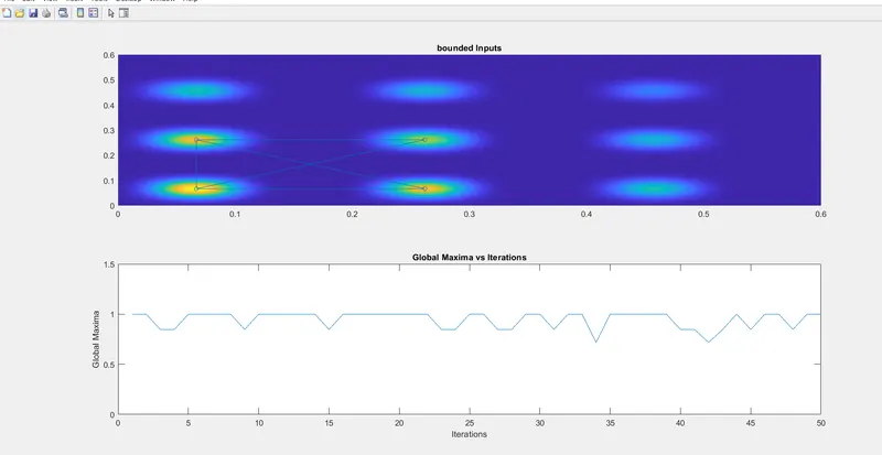
Results;
time taken: 13.1322
Programe code of case_3;
%case 3
% progrman to find global maxima using genetic algorthim

clear all
close all
clc
%1D Array _defining our search space
x = linspace(0,0.6,150);
y = linspace(0,0.6,150);
  num_cases = 250;

 %creating 2D array using meshgrid funciton

 [xx yy] = meshgrid(x,y);

 % study case no:1 Unbound inputs
for i = 1:length(xx)
    for j = 1:length(yy)
        input_vector(1) = xx(i,j);
        input_vector(2) = yy(i,j);
        f(i,j) = stalagmite(input_vector);

    end
end
%iterations of genetic algorthim

%defining population size

options = optimoptions('ga')
options = optimoptions(options,'PopulationSize',250)
tic
for i = 1:num_cases
    [inputs, fopt(i)] = ga(@stalagmite,2,[],[],[],[],[0;0],[0.6;0.6]); %bound inputs
    xopt(i) = inputs(1);
    yopt(i) = inputs(2);
end

study3_time = toc

figure (1)
subplot(2,1,1)
hold on
surfc(xx,yy,-f)
shading interp
plot3(xopt,yopt,-fopt,'marker','o','markersize',5)
title('bounded Inputs increased')
subplot(2,1,2)
plot(-fopt)
xlabel('Iterations')
ylabel('Global Maxima')
title('Global Maxima vs Iterations')
axis([0 50 0 1.5])
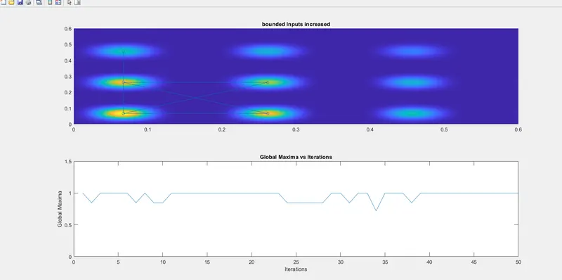
Results;
time takes; 57.9190
References;