Week 3 - Solving second order ODEs

Week 3- simple pendulum- application for second order ODE;

• Objective:

Write MATLAB code for simulation of a simple pendulum as solution for the second order equation.

• Pendulum Theory:

A simple pendulum consists of a ball (point-mass) m hanging from a (massless) string of length L and fixed at a pivot point P. When displaced to an initial angle and released, the pendulum will swing back and forth with periodic motion.

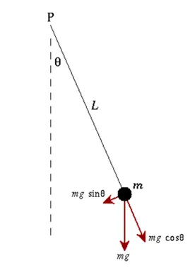
The Equation of Motion:

By applying Newton's second law for rotational systems, the equation of motion for the pendulum may be obtained

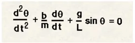
Where;

b = damping coefficient

L = length of the string in m

g = gravity in m/s2^2

m = mass in kg

Code 1 for the ODE function:

function[dtheta_dt] = ode_func(t,theta,b,g,l,m)
  
  theta1 = theta(1)  
  theta2 = theta(2)
  dtheta1_dt = theta2;   %first 1st order ode equation
  dtheta2_dt = -(b/m)*theta2 - (g/1)*sin(theta1);  %second 1st order ode equation 
  dtheta_dt = [dtheta1_dt ; dtheta2_dt];   % ; inside to use column matrix
end

Explanation:

We should define the differential equation before we start in the solution. And as far we know MATLAB cann’t solve the second order ODE, so we have to split the equation into two terms each term will be in a 1^st order ODE. “as shown in the CODE above”

Main Code for the pendulum motion:

clear all
close all
clc

%defining my inputs
b= 0.05;  %damping coefficient
g= 9.81;  %gravity 
l=1;       %length of the string
m=0.1;        %mass

% to solve the 1st ode we should define the intial coniditions for the
% displacment & velocity 

theta_0 = [0;3];     % 0 m for the displacment & 3 rad/s for  'velocity'

%time points
t_span = linspace(0,20,200);

%solve ODE

[t, results] = ode45(@(t,theta) ode_func(t,theta,b,g,l,m),t_span, theta_0);


plot(t,results(:,1))
hold on
plot(t,results(:,2))
ylabel('velocity')
xlabel('time')
legend('Displacement','Angular velocity')

%Animation

figure
ct=1;
for i=1:length(t)
    %coordinates
    %starting point of the string
    x0=0;
    y0=0;
    %end point
    x1=l*sin(results(i,1));
    y1=-l*cos(results(i,1));
    
   % plotting the mass or the bob
   
   plot([x0 x1],[y0,y1],'color', 'b');
   line([-1 1], [0,0],'linewidth',4,'color','r')
   hold on
   plot(x1,y1,'marker','o','markersize',20)
   %axis setting
   axis([-1.5 1.5 -2 2])
   grid on
   pause(0.03)
   M(ct)=getframe(gcf)
   ct=ct+1;
   hold off
end

movie(M)
videofile=VideoWriter('pendulum animation.avi','uncompressed AVI')
open(videofile)
writeVideo(videofile,M)
close(videofile)
    
  

Stepwise explanation:

1. As usual we start our program with the commands of; Clear all, Close all, Clc
2. Define our inputs of (g,l,m,b)
3. Time span of the pendulum is set by the linspace command
4. Theta value is given as a column matrix
5. Ode45 is the function solver used in MATLAB
6. Plot and line commands to create the graphs
7. Hold on command used to merge the previous plots with the next plots
8. Hold off is used to stop the command “hold on” and stop the merging of plots
9. Marker command is used to create the bob of the pendulum
10. For loop is used to help in getting more accurate simulation of the simple pendulum as we need to repeat the motion
11. Ct = counter command is used to make the values changes in each for loop
12. And videowriter used to create the video file

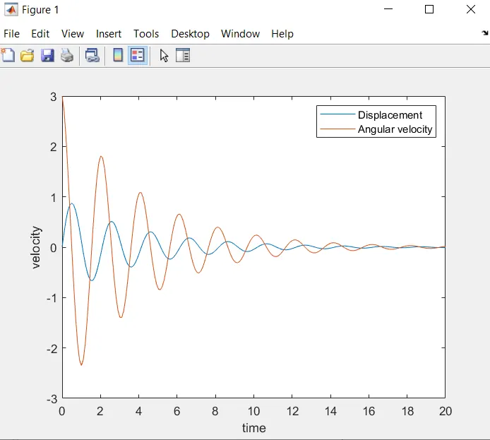
Result:

Plot is obtained between velocity and time

Video file link;

https://drive.google.com/file/d/1So4Uz0whJXxJW_BcuV7jdteqWjCiv8j7/view?usp=sharing