Week 4.1 - Genetic Algorithm

AIM :

To write a code in the MATLAB to optimize the stalagmite function and to find the global maxima of the function.

Theory :

A genetic algorithm is a search-based algorithm used for solving optimization problems.Genetic algorithms are commonly used to generate high-quality solutions to optimization and search problems by relying on biologically inspired operators as mutation, crossover and selection.It is inspired by Charles Darwin's theory of natural evolution. This algorithm reflects the process of natural selection where the fittest individuals are selected for reproduction to produce offspring of the next generation.

Genetic algorithms work process :

Genetic algorithms use the evolutionary generational cycle to produce high-quality solutions. They use various operations that increase or replace the population to provide an improved fit solution.

Genetic algorithms follow the following phases to solve complex optimization problems:

Initialization

The genetic algorithm starts by generating an initial population. This initial population consists of all the probable solutions to the given problem. The most popular technique for initialization is the use of random binary strings.

Fitness assignment

The fitness function helps in establishing the fitness of all individuals in the population. It assigns a fitness score to every individual, which further determines the probability of being chosen for reproduction. The higher the fitness score, the higher the chances of being chosen for reproduction.

Selection

In this phase, individuals are selected for the reproduction of offspring. The selected individuals are then arranged in pairs of two to enhance reproduction. These individuals pass on their genes to the next generation.

The main objective of this phase is to establish the region with high chances of generating the best solution to the problem (better than the previous generation). The genetic algorithm uses the fitness proportionate selection technique to ensure that useful solutions are used for recombination.

Reproduction

This phase involves the creation of a child population. The algorithm employs variation operators that are applied to the parent population. The two main operators in this phase include crossover and mutation.

1. Crossover: This operator swaps the genetic information of two parents to reproduce an offspring. It is performed on parent pairs that are selected randomly to generate a child population of equal size as the parent population.

2. Mutation: This operator adds new genetic information to the new child population. This is achieved by flipping some bits in the chromosome. Mutation solves the problem of local minimum and enhances diversification. The following image shows how mutation is done.

Replacement

Generational replacement takes place in this phase, which is a replacement of the old population with the new child population. The new population consists of higher fitness scores than the old population, which is an indication that an improved solution has been generated.

Termination

After replacement has been done, a stopping criterion is used to provide the basis for termination. The algorithm will terminate after the threshold fitness solution has been attained. It will identify this solution as the best solution in the population.

Working Procedure :

Initially stalagmite function is defined in a seperate script.

The negative sign is used in front of the function to obtain maxima of the function rather minima.

Nested for loop is utilized to iterate each of the elements

GA is used to determine the optimal of the function.

Plot is generated for different cases.

Three case consideration:

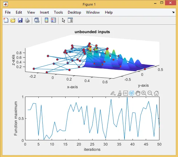
Unbounded inputs.

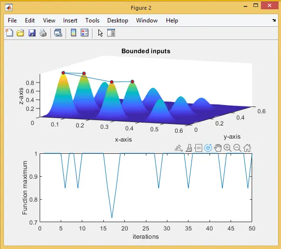
Bounded inputs - restricted with upper and lower bounds

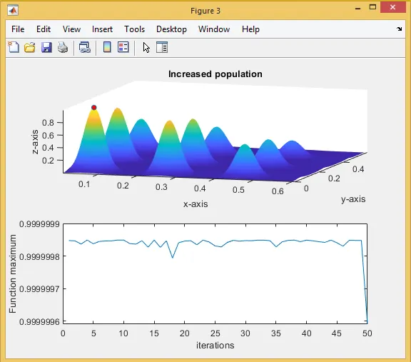
Bounded inputs with options - increasing no of iterations by giving population size.

Code :

Stalagmite Code :

function [f]=stalagmite(V)
x = V(1);
y = V(2);

f1x=(sin((5.1*pi*x)+0.5))^6;
f1y=(sin((5.1*pi*y)+0.5))^6;
f2x=exp(-4*log(2)*(((x-0.0667)^2)/0.64));
f2y=exp(-4*log(2)*(((y-0.0667)^2)/0.64));

f=-(f1x*f1y*f2x*f2y);

Main code :

 close all
 clear all
 clc
 % defining the search space
 x = linspace(0,0.6,150);
 y = linspace(0,0.6,150);
 % to create 2d mesh
%   [xx,yy] = meshgrid(x,y);
%  % assigning valus to inputs
  for i = 1:length(x)% takes values until length of xx
      for j = 1:length(y)% takes values until length of xx
          inputs(1) = x(i);
          inputs(2) = y(j);
          f(i,j) = stalagmite(inputs);
      end
  end
 num_case = 50; % creating a variable and assigning the number to which iterations performed
%  f = get_stalagmite(x,y);
 tic % Starts the timer
 % Studt case-1
 for z = 1:num_case % takes values until length of num_cases
         [inputs,fopt(z)]  = ga(@stalagmite,2);% solve stalagmite function using GA and assigning to variables
         xopt(z) = inputs(1);
         yopt(z) = inputs(2);
 end
 Time_study1 = toc % Gives time taken to perform the case

 figure(1)
 subplot(2,1,1) % creates sub-plot in the figure 
 hold on
 surfc(x,y,-f) % Creates a surface
 shading interp % varies the color in each line segment and face by interpolating the colormap index or true color value across the line or face.
 plot3(xopt,yopt,-fopt,'marker','o','markersize',5,'markerfacecolor','r')% plot3 command used to plot in 3 axis
 % marker is used to create a visible points on the plot
 title('unbounded inputs') 
 xlabel('x-axis')
 ylabel('y-axis')
 zlabel('z-axis')
 subplot(2,1,2)
 plot(-fopt)
 xlabel('iterations')
 ylabel('Function maximum')

% Study Case-2 Defining upper and lower bounds
tic
 for z = 1:num_case
         [inputs,fopt(z)] = ga(@stalagmite,2,[],[],[],[],[0;0],[0.4;0.4]);
         %defines a set of lower and upper bounds on the design variables
         xopt(z) = inputs(1);
         yopt(z) = inputs(2);
 end
 Time_study2 = toc

 figure(2)
 subplot(2,1,1)
 hold on
 surfc(x,y,-f)
 shading interp
 plot3(xopt,yopt,-fopt,'marker','o','markersize',5,'markerfacecolor','r')
 title('Bounded inputs')
 xlabel('x-axis')
 ylabel('y-axis')
 zlabel('z-axis')
 subplot(2,1,2)
 plot(-fopt)
 xlabel('iterations')
 ylabel('Function maximum')
 clc
 % Study Case-3 Increasing iterations
 options = optimoptions('ga');% returns a set of default options for the SolverName solver.
 options = optimoptions(options,'PopulationSize',270);%Defining population size
 
 tic
 for z = 1:num_case
         [inputs,fopt(z)]  = ga(@stalagmite, 2,[],[],[],[],[0;0],[0.4;0.4],[],[],options);
         % takes the values of options and solves ga in required population
         xopt(z) = inputs(1);
         yopt(z) = inputs(2);
 end
 Time_study3 = toc;

 figure(3)
 subplot(2,1,1)
 hold on
 surfc(x,y,-f)
 shading interp
 plot3(xopt,yopt,-fopt,'marker','o','markersize',5,'markerfacecolor','r')
 title('Increased population')
 xlabel('x-axis')
 ylabel('y-axis')
 zlabel('z-axis')
 subplot(2,1,2)
 plot(-fopt)
 xlabel('iterations')
 ylabel('Function maximum')
 % The Global Maximum at the position
%  display(inputs)

Result :

Thus a code to optimize the stalagmite function and to find the global maxima of the function in MATLAB is done.