Week 3 - Solving second order ODEs

AIM:

To write a program in Matlab to simulate the motion of simple pendulum by solving the second order Ordinary Differential Equation (ODE).

OBJECTIVE:

Solving the second order ODE which represents the equation of motion of a simple pendulum.

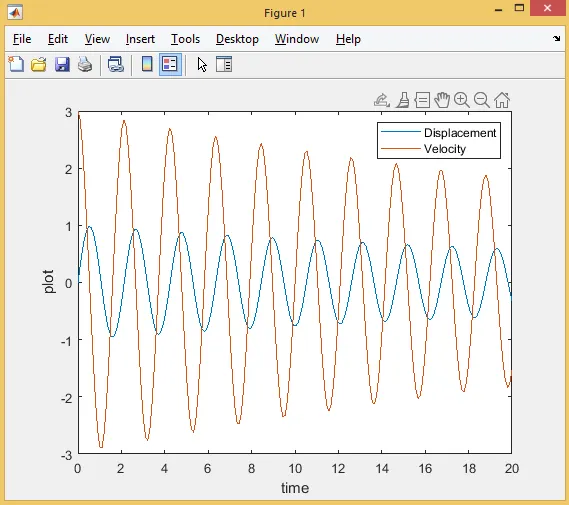
To plot the graph for Velocity and Displacement, depends on the change of Time.

To animate the motion of the simple pendulum.

PROJECT DEFINITION:

In this project we are going to discuss about the transient behaviour of the pendulum motion with the help of second order ODE by using ode45 which is the inbuilt solver in Matlab.

Simple Pendulum:

A Simple pendulum consists of a mass (m) small-diameter bob hanged with a non stretchable mass less string of length (L) fixed at one end. When the mass is moved to an initial displacement and released, then the pendulum will start to swing in the back and forth motion with the periodic interval of time under the influence of gravity. Pendulum is most commonly used in clocks.

ODE:

Ordinary Differential Equation contains only one independent variable and one or more of its derivatives with respect to the variable. The order of ODE is defined to be the order of the highest derivative that occur in the equation. In this the ODE is used to define the displacement and the velocity of the pendulum with respect to time. Second order ODE is used here to calculate the motion of the pendulum. In Matlab the function ode45 is used to solve the second order equation.

FORMULA:

The second order ODE for solving the motion of the pendulum is given below

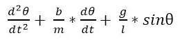
Hence,

g – acceleration due to gravity (m/s^2)

l – length of the string (m)

m – mass of the bob (kg)

b – damping coefficient (Nm/s)

θ – angle made between the fixed point to the bob moved

In order to solve the second order differential equation by using ode45 solver in Matlab, then the higher order differentia equation is to be converted into simple differential equation.

Therefore, by assuming the constant

θ = θ1

By applying above constants,

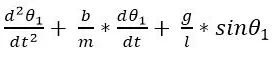
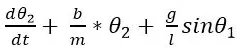
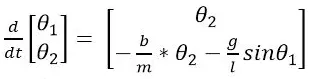
Simplified differential equation is written as

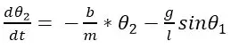
The matrix derivation of simple equation

The input variables to simulate the motion of the pendulum is given below as,

l = 1 m

m = 1 kg

b = 0.05

g = 9.81 m/s^2

Motion of the pendulum is to be simulated between 0-20 sec, for angular displacement = 0, angular velocity = 3 rad/sec at time t = 0.

INPUT CODE :

These simplified differential equations are used in the Matlab as a ode45 function file.

Main Code :

clear all
close all
clc

%Input parameters

b=0.05;      %damping co-efficient
g=9.81;      %acceleration due to gravity
l=1;         %length of the string  
m=1;         %mass of the bob

%Initial conditions 
theta_0=[0;3];
t_span=linspace(0,20,200);  %time span

%ode solver
[t,results]=ode45(@(t,theta) ode_func(t,theta,b,g,l,m), t_span,theta_0);

%Plotting results of displacements and velocity
figure(1)
plot(t,results(:,1))
hold on
plot(t,results(:,2))
xlabel('time')
ylabel('plot')
legend('Displacement','Velocity')
displacement = results(:,1);
velocity = results(:,2);

%Co-ordinates
x0=0;
y0=0;
ct=1;
%for loop to calculate the displacement of the bob
for i=1:length(displacement)
    x1=l*sin(displacement(i));
    y1=-l*cos(displacement(i));
 
% plot to animate the pendulum motion
    figure(2)
    plot([-1 1],[0 0],'linewidth',15,'color','b')                          %plot for the fixed beam   
    hold on
    plot(x0,y0,'o','markersize',10,'markerFacecolor','w','color','k')      %plot for the fixed point
    hold on
    plot([x0 x1],[y0 y1],'linewidth',3,'color','g')                        %plot for the string
    hold on
    plot(x1,y1,'o','markersize',15,'markerFacecolor','y','color','r')      %plot for the moving bob
    axis([-2 2 -2 2])
    M(ct)=getframe(gcf);
    ct=ct+1;
    hold off
end

movie(M)
videofile = VideoWriter('Simple_Pendulum.avi','uncompressed AVI');
open(videofile)
writeVideo(videofile,M)
close(videofile)

Function Code :

function[dtheta_dt]=ode_func(t,theta,b,g,l,m);
theta1=theta(1);
theta2=theta(2);
dtheta1_dt=theta2;
dtheta2_dt=-(b/m)*theta2-(g/l)*sin(theta1);
dtheta_dt=[dtheta1_dt;dtheta2_dt];
end

CODE EXPLANATION :

Main code explanation:

At the initial stage of the program the main inputs to define the pendulum is given like damping coefficient, length of string, mass of the bob.

Next the initial displacement and initial velocity of the pendulum is defined as the values of theta_0, then the oscillation time span of the pendulum is given.

Now the solver ode45 is used to solve the second order ODE to define the motion of the pendulum w.r.t to time.

In that, the function ode is called with the inputs are integrated, time span and initial condition.

Here the function is provided in the form of anonymous function. Thus the inputs are passed to that function, which do the operations of ODE and returns the values to the variable t and results as the output.

Thus the output results variable hold the values of displacement of the bob in first column and the values of velocity of the pendulum in second column.

Then the plot command is used to plot the graph of displacement and velocity of the pendulum.

In order to animate the motion of the pendulum, for loop is used to store the images of the pendulum at different time interval.

Now all the images are converted into the movie.

Function Code explanation:

The second order ODE is simplified into simple terms to calculate the unknown values.

Thus the anonymous function gets executed and gets the values of displacement and velocity.

Now the values are passed to the results variable.

OUTPUT :

The graph for Velocity and Displacement, depends on the change of Time for the pendulum is plotted below,

The pendulum set up is given below,

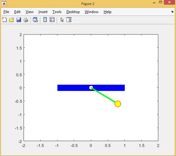
The animation of motion of the simple pendulum is given in below link,

https://drive.google.com/file/d/1iZKPeqOEiugP7CrThOcQBSpMNBGjFktB/view?usp=sharing

RESULT :

Thus the simulation of the motion of simple pendulum by solving the second order ODE is done by using the ode45 solver in Matlab.