Week 4.1 - Genetic Algorithm

genticalgorithm is a in built solver in matlab to find maximum or minimum vale.basically it is a optimisation technique.it is used by charles darvin's theory of natural evolution.

stalagmite function is to find maxima and minima (using -f and f)according to davine's theory.

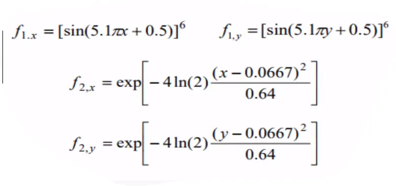
f=-f1x.f2x.f1y.f1y(we have to find maxima)

function [f]=stalagmite(input_vector)
x=input_vector(1)
y=input_vector(2)
f1_x=(sin(5.1*pi*x+0.5)).^6;
f1_y=(sin(5.1*pi*y+0.5)).^6;
b1=(x-0.0667).^2/(0.64);
b2=(y-0.0667).^2/(0.64);
f2_x=exp(-4*log(2)*b1);
f2_y=exp(-4*log(2)*b2);
f=-(f1_x*f2_x*f1_y*f2_y);
end

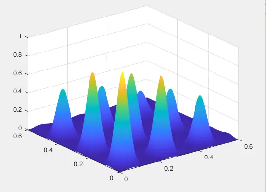
mesh grid is used for 3 dimensions between 0.6-x,0.6-y

Genetic algorithm solves smooth or nonsmooth optimization problems with any types of constraints, including integer constraints. It is a stochastic, population-based algorithm that searches randomly by mutation and crossover among population members.

[X,Y] = meshgrid(x,y) returns 2-D grid coordinates based on the coordinates contained in vectors x and y. X is a matrix where each row is a copy of x, and Y is a matrix where each column is a copy of y. The grid represented by the coordinates X and Y has length(y) rows and length(x) columns

ist case is natural selection.

2nd case is setting upper and lower bound(limits)

3rd case is defining initial poulation size.in orde to find best fit.

clear all
close all
clc
%defining our  space
x=linspace(0,0.6,150);
y=linspace(0,0.6,150);
% creating mesh
[xx,yy]=meshgrid(x,y);
num_cases=100;
%evaluating stalgmite function
for i=1:length(xx)
    for j=1:length(yy)
        input_vector(1)=xx(i,j);
        input_vector(2)=yy(i,j);
        f(i,j)=stalagmite(input_vector);
    end
end
figure(1)
surf(xx,yy,-f)
shading interp
[x,fval]=ga(@stalagmite,2)

tic
for i=1:num_cases
[inputs,fopt(i)]=ga(@stalagmite,2);
xopt(i)=inputs(1);
yopt(i)=inputs(2);
end
study1_time=toc
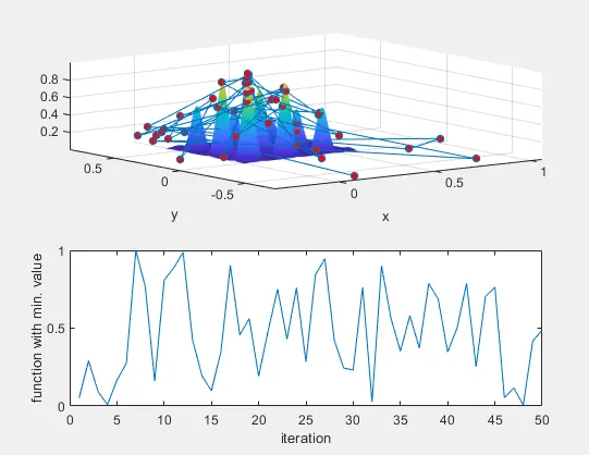
%plotting the graph
figure(2)
subplot(2,1,1)
surfc(xx,yy,-f);
hold on
shading interp
plot3(xopt,yopt,-fopt,'marker','o','markersize',5,'markerfacecolor','r');
xlabel('x')
ylabel('y')
grid on
subplot(2,1,2)
plot(-fopt)
xlabel('iteration')
ylabel('function with min. value')

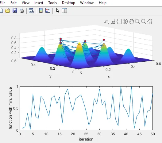
%statistical behaviour bounded
tic
for j=1:num_cases
    [inputs,fopt(j)]=ga(@stalagmite,2,[],[],[],[],[0;0],[1;1]);
    xopt(j)=inputs(1);
    yopt(j)=inputs(2);
end
study2_time=toc
%plotting the graph
figure(3)
subplot(2,1,1)
surfc(xx,yy,-f);
hold on
shading interp
plot3(xopt,yopt,-fopt,'marker','o','markersize',5,'markerfacecolor','r');
xlabel('x')
ylabel('y')
grid on
subplot(2,1,2)
plot(-fopt)
xlabel('iteration')
ylabel('function with min. value')
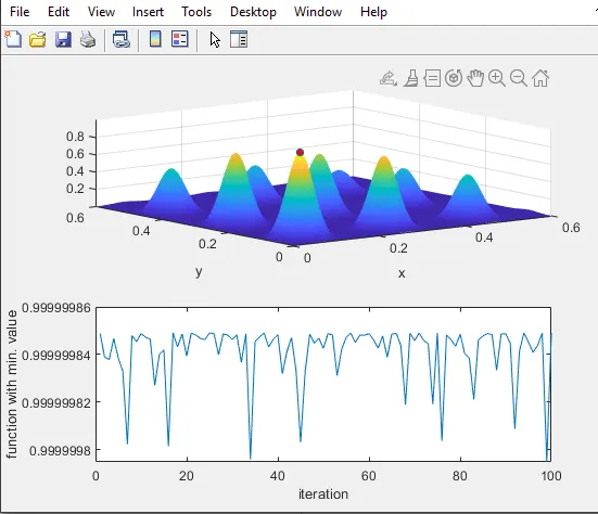
%statistical behaviour population best fit
tic
options=optimoptions("ga")
options=optimoptions(options,'populationSize',400)

for k=1:num_cases
    [inputs,fopt(k)]=ga(@stalagmite,2,[],[],[],[],[0;0],[0.1;0.1],[],[],options);
    xopt(k)=inputs(1);
    yopt(k)=inputs(2);
end
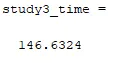
study3_time=toc
%plotting the graph
figure(4)
subplot(2,1,1)
surfc(xx,yy,-f);
hold on
shading interp
plot3(xopt,yopt,-fopt,'marker','o','markersize',5,'markerfacecolor','r');
xlabel('x')
ylabel('y')
grid on
subplot(2,1,2)
plot(-fopt)
xlabel('iteration')
ylabel('function with min. value')