Week 4.1 - Genetic Algorithm
Objective- To optimize the stalagmite function to find the global maxima and code it in MATLAB.
Theory- what is stalagmite ? A stalagmite is a type of rock formation that rises from the floor of a cave due to the accumulation of material deposited on the floor from ceiling drippings.
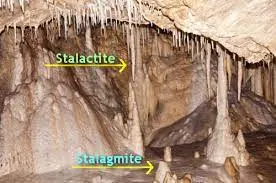
Similarly when we optimize a stalagmite function it outputs many local maximas and minimas and a global maxima and a global minima. To help us optimize this function we use genetic algorithm tool in matlab, but after 2015 the tool has been removed and now its ‘optimize live editor text box’. In this project we will be directly using genetic algorithm with its syntax instead of the live editor text box.
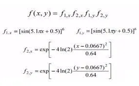
Stalagmite function-
What is genetic algorithm? Genetic algorithms are randomized search algorithms that have been developed in an effort to imitate the mechanics of natural selection and natural genetics. Genetic algorithm is a kind of stochastic algorithm based on the theory of probability. In application this method to a stagewise superstructure model, the search process is determined by stochastic strategy. The global optimal solution for the synthesis of heat exchanger networks can be obtained at certain probability. The search process begins with a set of initial stochastic solutions, which is called “population.” Each solution is called “chromosome,” the chromosome is composed of “gene,” and the “gene” stands for the optimal variables of heat exchanger networks, for example, the mass flowrates of cold streams and hot streams.
The genetic operation adopts the transferring principle of probability, selects some good chromosomes to propagate at certain probability, and lets the other inferior chromosomes to die; thus, the search direction will be guided to the most promising region
The strength of the genetic algorithm is the exploration of different regions of the search space in relatively short computation time. Furthermore, multiple and complex objectives can easily be included.

Syntax of ga(genetic algorithm)
- x = ga(fun,nvars)
- x = ga(fun,nvars,A,b)
- x = ga(fun,nvars,A,b,Aeq,beq)
- x = ga(fun,nvars,A,b,Aeq,beq,lb,ub)
- x = ga(fun,nvars,A,b,Aeq,beq,lb,ub,nonlcon)
- x = ga(fun,nvars,A,b,Aeq,beq,lb,ub,nonlcon,options)
- x = ga(fun,nvars,A,b,[],[],lb,ub,nonlcon,IntCon)
- x = ga(fun,nvars,A,b,[],[],lb,ub,nonlcon,IntCon,options)
- x = ga(problem)
- [x,fval] = ga(___)
- [x,fval,exitflag,output] = ga(___)
- [x,fval,exitflag,output,population,scores] = ga(___)
Description of each syntax
- x = ga(fun,nvars) finds a local unconstrained minimum, x, to the objective function, fun. nvars is the dimension (number of design variables) of fun.
- x = ga(fun,nvars,A,b) finds a local minimum x to fun, subject to the linear inequalities A*x ≤ b. ga evaluates the matrix product A*x as if x is transposed (A*x').
- x = ga(fun,nvars,A,b,Aeq,beq) finds a local minimum x to fun, subject to the linear equalities Aeq*x = beq and A*x ≤ b. (Set A=[] and b=[] if no linear inequalities exist.) ga evaluates the matrix product Aeq*x as if x is transposed (Aeq*x').
- x = ga(fun,nvars,A,b,Aeq,beq,lb,ub) defines a set of lower and upper bounds on the design variables, x, so that a solution is found in the range lb ≤ x ≤ ub. (Set Aeq=[] and beq=[] if no linear equalities exist.)
- x = ga(fun,nvars,A,b,Aeq,beq,lb,ub,nonlcon) subjects the minimization to the constraints defined in nonlcon. The function nonlcon accepts x and returns vectors C and Ceq, representing the nonlinear inequalities and equalities respectively. ga minimizes the fun such that C(x) ≤ 0 and Ceq(x) = 0. (Set lb=[] and ub=[] if no bounds exist.)
- x = ga(fun,nvars,A,b,Aeq,beq,lb,ub,nonlcon,options) minimizes with the default optimization parameters replaced by values in options. (Set nonlcon=[] if no nonlinear constraints exist.) Create options using optimoptions.
- x = ga(fun,nvars,A,b,[],[],lb,ub,nonlcon,IntCon) or x = ga(fun,nvars,A,b,[],[],lb,ub,nonlcon,IntCon,options) requires that the variables listed in IntCon take integer values.
- x = ga(problem) finds the minimum for problem, a structure described in problem.
- [x,fval] = ga(___), for any previous input arguments, also returns fval, the value of the fitness function at x.
- [x,fval,exitflag,output] = ga(___) also returns exitflag, an integer identifying the reason the algorithm terminated, and output, a structure that contains output from each generation and other information about the performance of the algorithm.
- [x,fval,exitflag,output] = ga(___) also returns exitflag, an integer identifying the reason the algorithm terminated, and output, a structure that contains output from each generation and other information about the performance of the algorithm.
Since stalagmite function outputs global minima so in the programming of the function we use f = -f1 to inverse the graph.
clear all
close all
clc

% defining search space
x = linspace(0,0.6,150);
y = linspace(0,0.6,150);

% creating mesh
[xx yy] = meshgrid(x,y);

% evaluating stalagmite
for i = 1:length(xx)
    for j = 1:length(yy)
        input_vector(1) = xx(i,j);
        input_vector(2) = yy(i,j);
        f(i,j) = stalagmite(input_vector);
    end
end

surfc(xx,yy,f)

shading interp

[inputs fval] = ga(@stalagmite, 2);
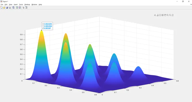
surface render of stalagmite function optimized by genetic algorithm
code of ga with three case studies
clear all
close all
clc

% defining search space
x = linspace(0,0.6,150);
y = linspace(0,0.6,150);
num_cases = 50;

% creating mesh
[xx yy] = meshgrid(x,y);

% evaluating stalagmite
for i = 1:length(xx);
    for j = 1:length(yy);
        input_vector(1) = xx(i,j);
        input_vector(2) = yy(i,j);
        f(i,j) = stalagmite(input_vector);
    end
end

% study 1

tic
for i= 1:num_cases;
    [inputs,fopt1(i)] = ga(@stalagmite,2);
    xopt1(i) = inputs(1);
    yopt1(i) = inputs(2);
end

study_time1 = toc;

% plotting
figure(1)
subplot(2,1,1);
hold on
surfc(xx,yy,f);
shading interp;

ylabel('y data');
xlabel('x data');
plot3(xopt1,yopt1,fopt1,'marker','o','markersize',5,'markerfacecolor','y')
title('unbounded inputs')
subplot(2,1,2);
plot(fopt1)
xlabel('iterations')
ylabel('maximum function')

% study 2 bounded values

tic
for i = 1:num_cases;
    [inputs,fopt2(i)] = ga(@stalagmite,2,[],[],[],[],[0;0],[1;]);
    xopt2(i) = inputs(1)
    yopt2(i) = inputs(2)
end
study_time2 = toc;

figure(2)
subplot(2,1,1);
hold on
surfc(xx,yy,f);
shading interp;

ylabel('y data');
xlabel('x data');
plot3(xopt2,yopt2,fopt2,'marker','o','markersize',5,'markerfacecolor','y')
title('bounded values')
subplot(2,1,2);
plot(fopt2)
xlabel('iterations')
ylabel('maximum function')

% study 3 bounding values, increasing population size

options = optimoptions('ga');
options = optimoptions(options,'populationsize',300);
tic
for i = 1:num_cases;
    [inputs,fopt3(i)] = ga(@stalagmite,2,[],[],[],[],[0;0],[1;1],[],[],options);
    xopt3(i) = inputs(1);
    yopt3(i) = inputs(2);
end

study_time3 = toc;

figure(3)
subplot(2,1,1);
hold on
surfc(xx,yy,f);
shading interp;

ylabel('y data');
xlabel('x data');
plot3(xopt3,yopt3,fopt3,'marker','o','markersize',5,'markerfacecolor','y')
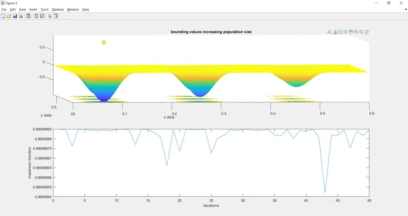
title('bounding values increasing population size')
subplot(2,1,2);
plot(fopt3)
xlabel('iterations')
ylabel('maximum function')
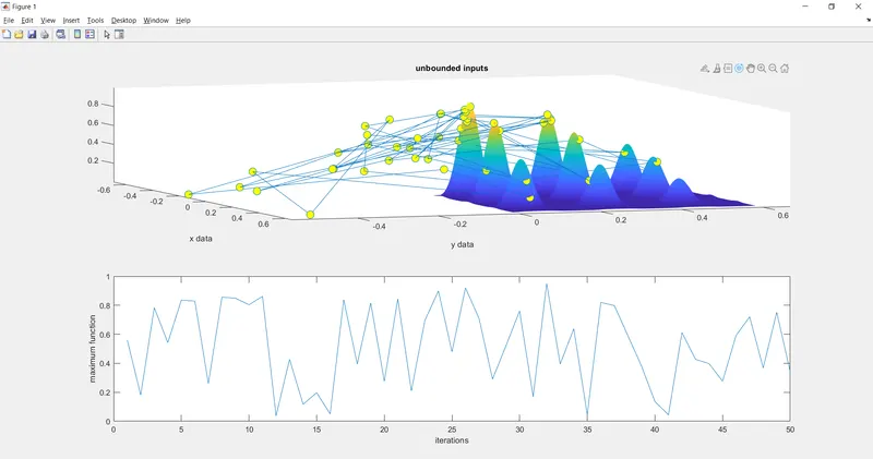
plots for the 3 studies
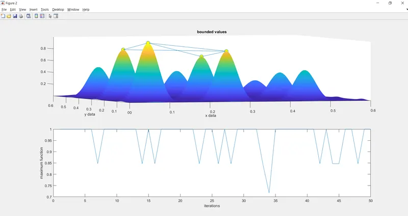
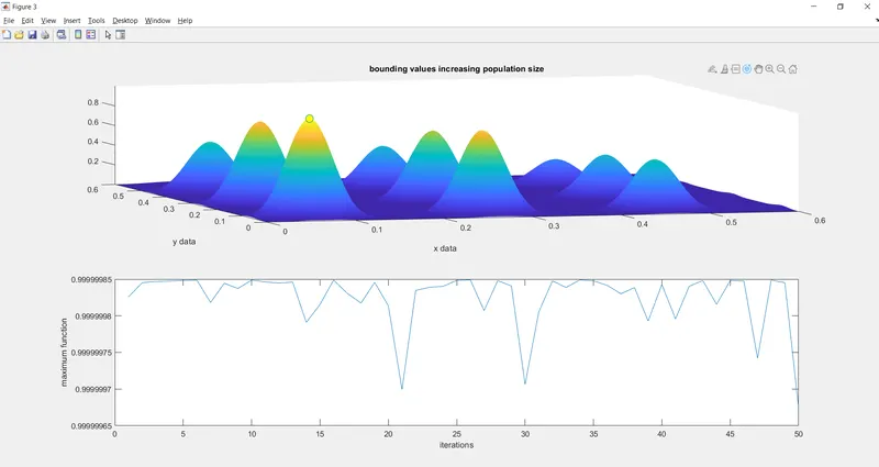
errors
minor syntax errors and errors with placing the negative sign in plot functions which lead to inverted surface projections.
references
Find minimum of function using genetic algorithm - MATLAB ga - MathWorks India