Challenge

Week 4.1 - Genetic Algorithm

SS Ashish Kumar17 Jul 2021

MATLAB

1.Aim:

To carry out optimization of a given data using a Genetic Algorithm(GA) in MATLAB.

2.Objectives:

To write a program in MATLAB that would optimize the stalagmite function and find its global maxima.
To plot all the relevant plots for different optimization studies.

3.Principles Involved:

A genetic algorithm (GA) is a method for solving both constrained and unconstrained optimization problems based on a natural selection process that mimics biological evolution. The algorithm repeatedly modifies a population of individual solutions. At each step, the genetic algorithm randomly selects individuals from the current population and uses them as parents to produce the children for the next generation. Over successive generations, the population "evolves" toward an optimal solution. The genetic algorithm is applied to solve problems that are not well suited for standard optimization algorithms, including problems in which the objective function is discontinuous, nondifferentiable, stochastic, or highly nonlinear.
The genetic algorithm uses three main types of rules at each step to create the next generation from the current population:
- Selection rules select the individuals, called parents, that contribute to the population at the next generation.
- Crossover rules combine two parents to form children for the next generation.
- Mutation rules apply random changes to individual parents to form children.
The genetic algorithm differs from a classical, derivative-based, optimization algorithm in two main ways, as summarized in the following table.

Genetic Algorithms(GAs) are adaptive heuristic search algorithms that belong to the larger part of evolutionary algorithms. Genetic algorithms are based on the ideas of natural selection and genetics. These are intelligent exploitation of random search provided with historical data to direct the search into the region of better performance in solution space. They are commonly used to generate high-quality solutions for optimization problems and search problems.
Genetic algorithms simulate the process of natural selection which means those species who can adapt to changes in their environment can survive and reproduce and go to the next generation. In simple words, they simulate “survival of the fittest” among individuals of consecutive generations for solving a problem. Each generation consist of a population of individuals and each individual represents a point in search space and possible solution. Each individual is represented as a string of character/integer/float/bits. This string is analogous to the Chromosome.

Foundation of Genetic Algorithms: Genetic algorithms are based on an analogy with the genetic structure and behavior of chromosomes of the population. Following is the foundation of GAs based on this analogy –

The individual in population compete for resources and mate
Those individuals who are successful (fittest) then mate to create more offspring than others
Genes from the “fittest” parent propagate throughout the generation, that is sometimes parents create offspring which is better than either parent.
Thus each successive generation is more suited for their environment.

Search Space: The population of individuals is maintained within search space. Each individual represents a solution in search space for a given problem. Each individual is coded as a finite length vector (analogous to chromosome) of components. These variable components are analogous to Genes. Thus a chromosome (individual) is composed of several genes (variable components).
Fitness Score: A Fitness Score is given to each individual which shows the ability of an individual to “compete”. The individual having optimal fitness score (or near-optimal) is sought.
The GAs maintains the population of n individuals (chromosome/solutions) along with their fitness scores. The individuals having better fitness scores are given more chances to reproduce than others. The individuals with better fitness scores are selected who mate and produce better offspring by combining chromosomes of parents. The population size is static so the room has to be created for new arrivals. So, some individuals die and get replaced by new arrivals eventually creating a new generation when all the mating opportunity of the old population is exhausted. It is hoped that over successive generations better solutions will arrive while at least fit die.

Each new generation has on average more “better genes” than the individual (solution) of previous generations. Thus each new generations have better “partial solutions” than previous generations. Once the offspring produced having no significant difference from offspring produced by previous populations, the population is converged. The algorithm is said to get converged to a set of solutions for the problem.
Operators of Genetic Algorithms Once the initial generation is created, the algorithm evolve the generation using the following operators –
1) Selection Operator: The idea is to give preference to the individuals with good fitness scores and allow them to pass their genes to successive generations.
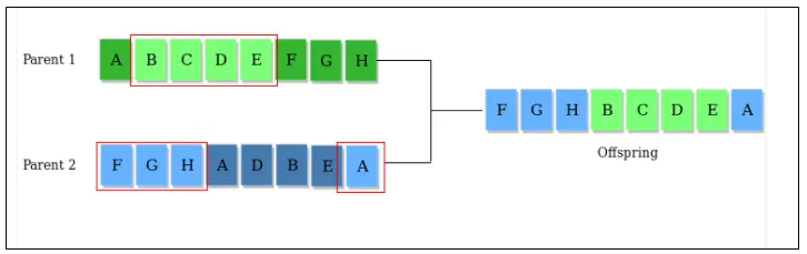
2) Crossover Operator: This represents mating between individuals. Two individuals are selected using a selection operator and crossover sites are chosen randomly. Then the genes at these crossover sites are exchanged thus creating a completely new individual (offspring). For example –

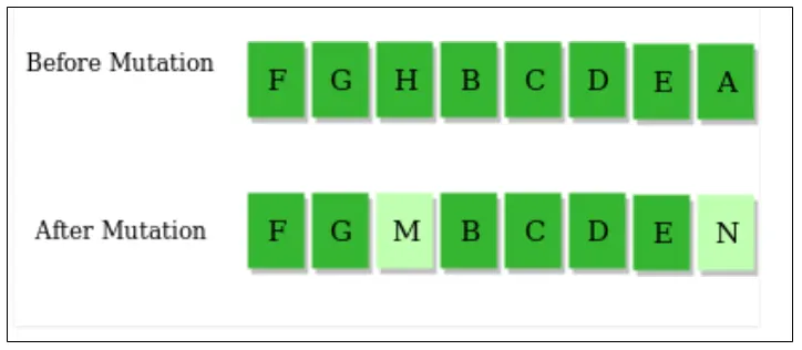
3) Mutation Operator: The key idea is to insert random genes in offspring to maintain the diversity in the population to avoid premature convergence. For example –

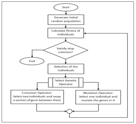
To sum the below-mentioned working principle of a Genetic Algorithm, neatly explained in the form of a flowchart.

4. Problem Definition:

A MATLAB program is to be developed which accurately performs optimization of a given set of data using a Genetic algorithm (GA). The inbuilt function employed to carry out this task is called the 'Stalagmite Function'. This function optimizes a given set of data provided by the user by using the fundamentals of a genetic algorithm.

In the Following code, three separate approaches are investigated and studied namely 'unbounded', 'Bounded with upper and lower limits', and ' Increased number of GA iterations.

5. MATLAB Code:

I. Stalagmite function: This function would carry out the optimization of the data provided by the user using the concept of GA

function [F]=stalagmite(input_vector)
x=input_vector(1);
y=input_vector(2);
f1=(sin(5.1*pi*x+0.5))^6;
f2=(sin(5.1*pi*y+0.5))^6;
f3=exp(-4*log(2)*((x-0.0667)^2/0.64));
f4=exp(-4*log(2)*((y-0.0667)^2/0.64));
F=-1*(f1*f2*f3*f4);
end

II. This is the main program that would call the Stalagmite function and find the global maxima among the data points.

clc%clears the screen
clear all%clears all variables
close all%closes all plots



%defining our search space 
x=linspace(0,0.6,150);%x is 1 1-d input array
y=linspace(0,0.6,150);%y is 1-d input array
num_cases=50;%number of iterations
[xx yy]=meshgrid(x,y);%creating a 2dimensional mesh
%for loop calls the stalagmite function
for i=1:length(xx)
    for j=1:length(yy)
        input_vector(1)=xx(i,j);
        input_vector(2)=yy(i,j);
        F(i,j)=stalagmite(input_vector);

    end
end





%____________Study-1-Statistical Behaviour-Unbounded_______________________
%**************************************************************************
tic
for i=1:num_cases%this loop runs for a maximum of 50 times
    [inputs1,fopt1(i)]=ga(@stalagmite,2);
    xopt1(i)=inputs1(1);
    yopt1(i)=inputs1(2);
end
study_1_time=toc%tic and toc commands calculate the time taken for execution of loop

figure(1)%1st figure window created
subplot(2,1,1)%multiple plots are created in same figure,2x1 order of plots and 1st is made current
surfc(xx,yy,-F)%draws a contour plot beneath the surface
hold on
shading interp%shades the plot by removing the mesh lines
plot3(xopt1,yopt1,-fopt1,'marker','o','markersize',5,'markerfacecolor','r')%makes a 3d plot
title('Unbounded Inputs')%title of the plot
xlabel('X-axis')
ylabel('Y-axis')
zlabel('Value of the function')
subplot(2,1,2)%multiple plots are created in same figure,2x1 order of plots and 2nd is made current
plot(-fopt1)
xlabel('Iterations')
ylabel('Function Maxima')




%_______Study-2-Statistical Behaviour with upper and lower bounds__________
%**************************************************************************
tic
for i=1:num_cases%this loop runs for a maximum of 50 times
    [inputs2,fopt2(i)]=ga(@stalagmite,2,[],[],[],[],[0;0],[0.5;0.5]);
    xopt2(i)=inputs2(1);
    yopt2(i)=inputs2(2);
end
study_2_time=toc%tic and toc commands calculate the time taken for execution of loop

figure(2)%2nd figure window created
subplot(2,1,1)%multiple plots are created in same figure,2x1 order of plots and 1st is made current
surfc(xx,yy,-F)%draws a contour plot beneath the surface
hold on
shading interp%shades the plot by removing the mesh lines
plot3(xopt2,yopt2,-fopt2,'marker','o','markersize',5,'markerfacecolor','r')%makes a 3d plot
title('Bounded Inputs')%title of the plot
xlabel('X-axis')
ylabel('Y-axis')
zlabel('Value of the function')
subplot(2,1,2)%multiple plots are created in same figure,2x1 order of plots and 2nd is made current
plot(-fopt2)
xlabel('Iterations')
ylabel('Function Maxima')


%_____________Study-3-Increasing the number of GA iterations_______________
%**************************************************************************

options=optimoptions('ga','PopulationSize',400)
tic
for i=1:num_cases%this loop runs for a maximum of 50 times
    [inputs3,fopt3(i)]=ga(@stalagmite,2,[],[],[],[],[0;0],[0.5;0.5],[],[],options);
    xopt3(i)=inputs3(1);
    yopt3(i)=inputs3(2);
end
study_3_time=toc%tic and toc commands calculate the time taken for execution of loop

figure(3)%3rd figure window created
subplot(2,1,1)%multiple plots are created in same figure,2x1 order of plots and 1st is made current
surfc(xx,yy,-F)%draws a contour plot beneath the surface
hold on
shading interp%shades the plot by removing the mesh lines
plot3(xopt3,yopt3,-fopt3,'marker','o','markersize',5,'markerfacecolor','r')%makes a 3d plot
title('Bounded Inputs with a population size of 400')%title of the plot
xlabel('X-axis')
ylabel('Y-axis')
zlabel('Value of the function')
subplot(2,1,2)%multiple plots are created in same figure,2x1 order of plots and 2nd is made current
plot(-fopt3)
xlabel('Iterations')
ylabel('Function Maxima')
% total_time=study_1_time+study_2_time+study_3_time

6. Explanation of the MATLAB code:

I. Study-1-Statistical Behaviour-Unbounded

Firstly we will create our own function to calculate the value of the objective function at various values of x and y.we use linspace command for creating various x and y values
Now, we create a matrix using the meshgrid function
Now the values in the different matrices created can be put as an input into the function that we have created, by calling it. By this, we can get the value of the function at various values of x and y.
since we have got the value of the function at various values, we now need to calculate the maximum value, which can be calculated using the ga, which is an in-built function
So, for our first study, we will use the for loop and iterate it 50 times We will use the following syntax here the number of variables is 2 that is x and y
In inputs we will get a 1*2 matrix for each iteration, it will basically give the value of x and y and fopt will give the optimum value of the function at these x and y values. These inputs can be stored and we can use the surf command to create a surface to visualize the function
We can also use the marker command to find the points of local maximum tic toc command can be used to look at the time taken for evaluation

II. Study-2-Statistical Behaviour-with Upper and Lower bounds

The drawback of this study is that since the GA command does not know the bound of these x and y values, so it can take the values greater than 0.6 or less than 0. So to overcome this we need to set up a second study that can put restrictions on the value of x and y. Hence we set up upper and lower bounds for this ga function and the syntax is
Where

lb is the lower bound and ub is the upper bound

A -linear inequality constraints b-linear inequality constraints Aeq-linear equality constraints beq-linear equality constraints

since there is no inequality constraints or equality constraints,A,b,Aeq,beq are represented as
If we execute the loop we will get different local maxima with bounded inputs.

III. Study-3-Statistical Behaviour-Increasing the number of GA iterations

But still, this is not correct as it is showing local maxima, but it is certainly better than the first study.
So to overcome this problem we need to increase the population size as it increases the probability to converge to a global maximum

The syntax that needs to be used is: This study can help us to converge to the most accurate solution
For ease of understanding abundant comment lines are provided within the code itself to better illustrate the concepts.

7. Results and Conclusions:

I. Study-1-Statistical Behaviour-Unbounded

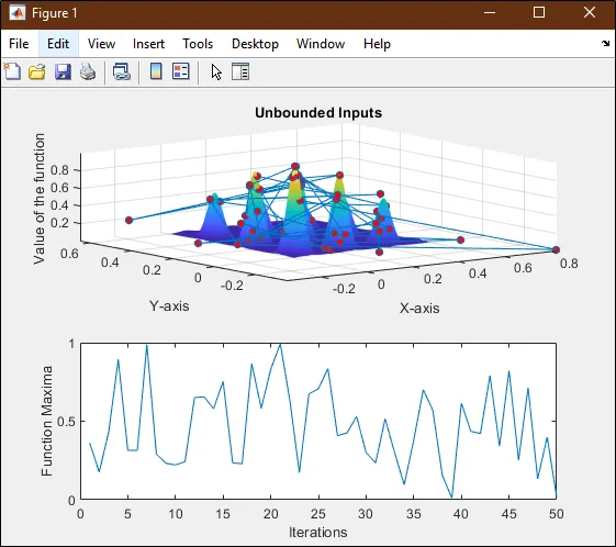
In this study, the GA handles unbounded data as a result, several local maxima (outside the stalagmite function) are predicted in course of the 50 iterations which are attempted. The local maximum change with every iteration, therefore it is safe to say that it is a low-accuracy analysis.

II. Study-2-Statistical Behaviour-with Upper and Lower bounds

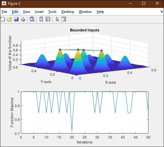
In this study, the accuracy is improved due to bound optimization as clearly evident from the figure above. The range within which the maxima lies is more clear in this study.

It is also inferred that even if we define a particular search space for GA, it doesn't run within the search space. So upper and lower bounds are pivotal to execute GA within a specified range.

III. Study-3-Statistical Behaviour-Increasing the number of GA iterations

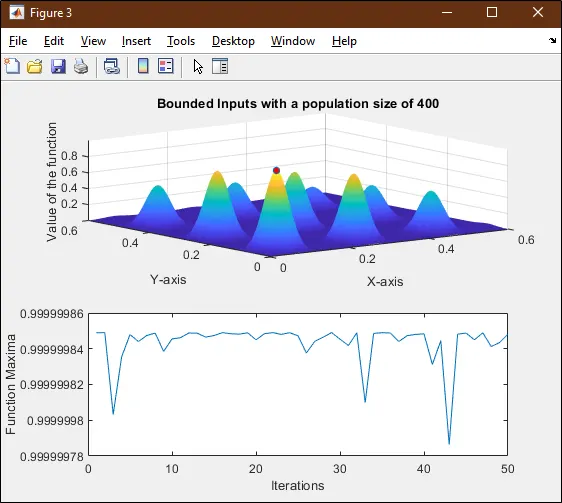
In this study, the GA predicts only one maximum which is the global maxima for the stalagmite function, hence by bounding i.e fixing the limits and increasing the population size we can increase the accuracy of the GA.

8. Errors faced during coding and steps undertaken to overtake them:

I. optimoptions command needs to be operated with the correct syntax

The correct use of 'optimoptions' in our case is :

options=optimoptions('ga','PopulationSize',400).

Any deviation from this syntax will lead to error(as shown below)

II. All commands and functions are case-sensitive

Incorrect usage of upper and lower cases in the code can lead to errors as below:

9.References:

Week 4.1 - Genetic Algorithm

Ship work like this
in your own course.

Talk to a career counsellor

Ship work like thisin your own course.

Talk to a career counsellor

Ship work like this
in your own course.