Week 3 - Solving second order ODEs
1. Aim:
To write a program in MATLAB that can simulate the transient behavior of a simple pendulum.
2. Objectives:
- To plot the variation of angular velocity & angular displacement of the pendulum with respect to time.
- To animate the damped motion of the pendulum.
3. Principles Involved:
I. Simple Pendulum:
- A pendulum is a weight suspended from a pivot so that it can swing freely. When a pendulum is displaced sideways from its resting, equilibrium position, it is subject to a restoring force due to gravity. that will accelerate it back toward the equilibrium position. When released, the restoring force acting on the pendulum's mass causes it to oscillate about the equilibrium position, swinging back and forth. The time for one complete cycle, a left swing, and a right swing is called the period. The period depends on the length of the pendulum and also to a slight degree on the amplitude, the width of the pendulum's swing. The word "pendulum" is new Latin, from the Latin pendulus, meaning 'hanging'.
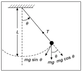
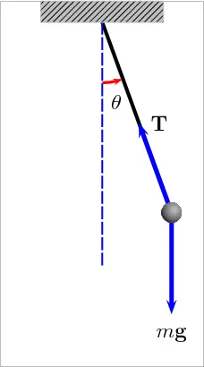
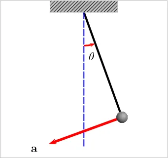
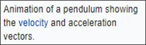
- The simple pendulum is a mechanical system that moves in an oscillatory motion. It consists of a point mass ‘m’ suspended by means of a light inextensible string of length L from fixed support as shown below The dimensions of the massive body are assumed to be so small concerning the length L of the string that it can be modeled as a particle with mass m. T. The motion occurs in a vertical plane and is driven by a gravitational force. The forces which are acting on the mass are shown in the figure. The tangential component of the gravitational force, mg sin θ, always acts towards the mean position θ = 0 opposite to the displacement, restoring force acting tangent to the arc
II. Ordinary Differential Equations(ODEs):
- In mathematics, an ordinary differential equation (ODE) is a differential equation containing one or more functions of one independent variable and the derivatives of those functions. The term ordinary is used in contrast with the term partial differential equation which may be with respect to more than one independent variable.
- Ordinary differential equations (ODEs) arise in many contexts of mathematics and social & natural sciences. Mathematical descriptions of change use differentials and derivatives. Various differentials, derivatives, and functions become related via equations, such that a differential equation is a result that describes dynamically changing phenomena, evolution, and variation. Often, quantities are defined as the rate of change of other quantities (for example, derivatives of displacement with respect to time), or gradients of quantities, which is how they enter differential equations.
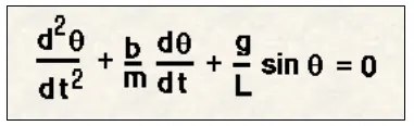
- Countless ODEs describe the physical phenomena of mechanical systems. One such Phenomenon called the 'Transient or Damped Motion of a Simple Pendulum' is mathematically represented by the ODE mentioned below & is derived from Newton's 2nd Law of Motion.
where:
`theta`= angular displacement of the pendulum during its motion with respect to its mean position in Rad`
't' is the time taken simple pendulum in Sec
'm' is the mass of the ball/bob in Kg
'b' is Damping Coefficient in Ns/m
'g' is the acceleration due to gravity (9.8 m/s^2)
'L' length of the string in m
Assuming,
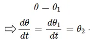
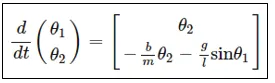
and writing the entire equation in matrix form we have,
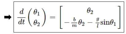
The solution of the above gives us the angular displacement which in turn can be used to determine the angular velocity and acceleration.
4. Problem Definition:
A MATLAB program is to be developed which accurately simulates the transient behavior ( due to damping) of a simple pendulum. The program should also be able to plot the variation of angular displacement & velocity with respect to time and animate the motion.
5. MATLAB Code:
I. Function which would properly define the ODE that represents the damped motion of pendulum:
function [dheta_dt]=ode_func(t,theta,b,g,l,m)
theta1=theta(1)
theta2=theta(2)
dtheta1_dt=theta2;
dtheta2_dt= -(b/m)*theta2-(g/l)*sin(theta1);
dheta_dt=[dtheta1_dt; dtheta2_dt];
end
II. This program would call the aforementioned program and then draw the plot & animate the results:
%This program solves the 2nd order ODE of a damped simple pendulum
clc
clear all
close all
%input parameters
b=0.05;%damping coefficient in N-S/m
g=9.81;%accleration due to gravity in m/s^2
l=1;%length of the pendulum string in mtrs
m=0.1;%mass of the ball in kg
%initial condition
theta_0=[0;3];%the initial angular displacement is 0 rad and initial angular velocity is 3 rad/s
%time points
t_span=linspace(0,20,500);%a time span of 20 seconds is created with 500 steps
%solving the ODE
[t,results]=ode45(@(t,theta) ode_func(t,theta,b,g,l,m), t_span ,theta_0);
%plotting the results
figure(1)
plot(t,results(:,1),'linewidth',2.5)%plots the angular displacement
hold on
grid on
plot(t,results(:,2),'linewidth',2.5)%plots the angular velocity
title('Damped Oscillation of a Simple Pendulum')
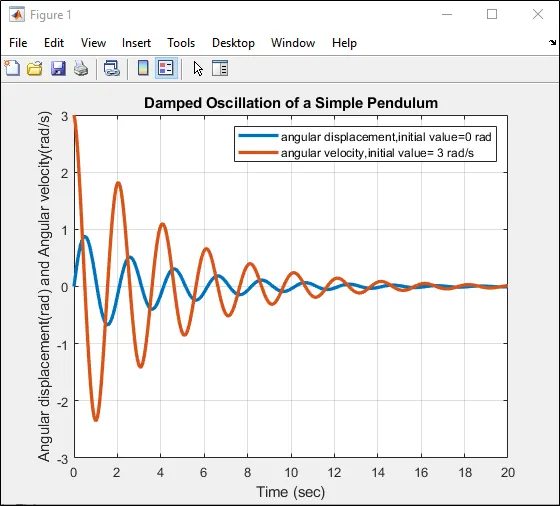
legend('angular displacement,initial value=0 rad','angular velocity,initial value= 3 rad/s')
ylabel('Angular displacement(rad) and Angular velocity(rad/s)')
xlabel('Time (sec)')
%animation of the pendulum
cntr=1;%this is 'for' loop's counter variable . 'cntr' is initialised to 1
for i=l:length(t)
x_i=0;%initial x-coordinate of the ball
y_i=0;%initial y-coordinate of the ball
x_f=l*sin(results(i,1));%final x-coordinate of the ball
y_f=-l*cos(results(i,1));%final y-coordinate of the ball
figure(2)%specifies a new figure window without altering the 1st fig window
plot([x_i x_f],[y_i y_f],'linewidth',3,'color','r')
title('Damped oscillation of a simple pendulum')
hold on
grid on
plot(x_f,y_f,'.','markersize',80,'color','b');%the ball is created
legend('pendulum string','pendulum ball')
axis([-1 1 -1 0.5]) % x &y limits in the plot are defined
hold off
pause(0.01)%to have a good viewing experience
M(cntr)=getframe(gcf);%captures each frame drom the 'cntr' loop counter variable
cntr=cntr+1;
end
%making a animation movie and saving it
%carful: commands are case sensitive
movie(M)
videofile=VideoWriter('simple_pendulum.avi','uncompressed AVI');%a video file of the name 'simple_pendulum.avi' is saved in the workin directory
open(videofile)
writeVideo(videofile,M)
close(videofile)
6. Explanation of the MATLAB code:
In this code the concept of ‘function call’ is neatly implemented. Firstly, a separate user-defined function is created titled ‘ode_func’. This function correctly represents the mathematical behavior of a simple pendulum when its amplitude of motion is gradually reducing due to the effect of damping. This function basically writes an ODE that properly encapsulates the damped behavior of the pendulum. This function takes several parameters like time, angular displacement, damping coefficient, acceleration due to gravity, length of the pendulum string, and the mass of the ball as input arguments. The variation of angular displacement with respect to time in the presence of all the aforementioned parameters is the output argument.
In the Main program, the values of the aforementioned 'input' parameters are provided along with initial displacement and velocity. The total time span of the motion is also supplied to this program. The user-defined function is now called by the main program through 'ode45' ( a MatLab solver for ODEs). Subsequently, the plot to elucidate the variation of angular displacement and velocity with respect to time is drawn and motion animated and captured in an avi file.
For ease of understanding abundant comment lines are provided within the code itself to better illustrate the concepts.
7. Results and Conclusions:
- The Plot to portray the transient behavior of the simple pendulum is shown below. Gradually over time, the amplitude of motion diminishes and eventually dies out completely. This is attributed to the presence of damping.
- Various frames are properly captured and compiled neatly into a video file. The link to the video is:
The animation properly illustrates the transient behavior of a simple pendulum.
8. Errors faced during coding and steps undertaken to overtake them:
I. Use of 'hold off' command:
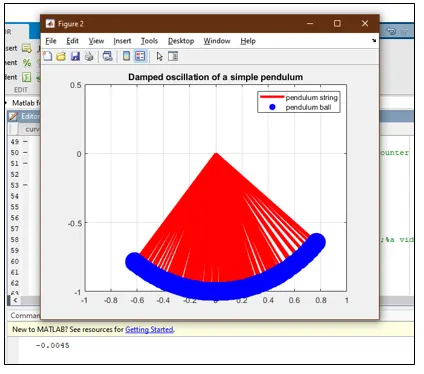
'hold off' command is necessary while capturing animations otherwise an improper animation as shown below is expected.
II. Use of 'axis' command:
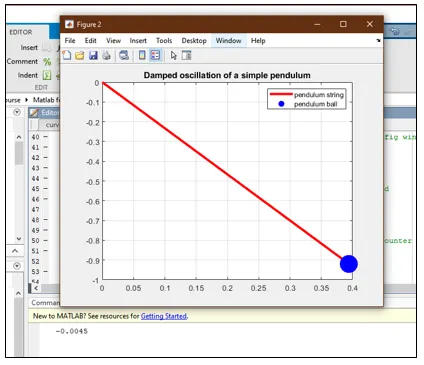
If the limits of the axes are not defined correctly by the 'axis' command then an improper plot as shown below is expected.
III. Commands used to write the animation movie are case sensitive:
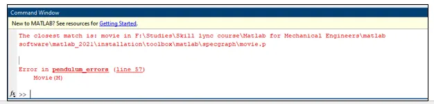
Utmost care is to be taken while writing the syntax to make the animation video as few commands like 'Movie', ‘writeVideo’, ‘VideoWriter’ have hybrid case structuring i.e they comprise of both upper and lower case alphabets. Failure to comply with this syntax can lead to error as shown below:
IV. 'Pause' Command:
Pause’ command is to be judiciously used. Different pause times can be tried to better animate the results. Technically speaking, this is not an error but prior knowledge of it could come in handy.
9. References:
- https://en.wikipedia.org/wiki/Pendulum
- https://www.sciencedirect.com/science/article/pii/B9781845695187500026
- https://www.mathworks.com/help/symbolic/simulate-physics-pendulum-swing.html
- https://skill-lync.com/knowledgebase/understanding-anonymous-functions-in-matlab-2
- https://skill-lync.com/knowledgebase/understanding-ode45-2