Week 4.1 - Genetic Algorithm

AIM : To calculate the global maxima of a stalagmite function using MATLAB.

OBJECTIVES:
1)To optimize the stalagmite function.
2)To determine the global maxima of the function.

THEORY: The global maxima of a stalagmite function can be obtained using a 'Gentic algorithm' in MATLAB.

GENETIC ALGORITHMS are a class of algorithms based on abstraction of darwin's evolution of biological systems , pioneered by holland. He was probably the first to use genetic operators such as the crossover and recombination, mutatation, and selection in the study of adaptive and artifical systems. Three main components or genetic operators in genetic algorithm are (.)crossover
(.)Mutation
(.)selection of the fittest

The genetic algorithm can be applied to solve a variety of optimizasation problems that are not well suite dfor standard optimization algorithms, including problems in which the objective function is discontinous ,non-differentiable ,stochastic or highly non linear.

PROCEDUERE:The following outline summarizes how the genetic algorithm works:
1. The algorithm begins by creating a random initial population.
2. The algorithm then creates a sequence of new population . At each step , the algorithm uses the individuals in the current generation to create the next population. To create the new population , the algorithm performs the following steps:
a) scores each member of the current population by computing its fitness value. These values are called the raw fitness scores.
b) scales the raw fitness scores to convert them into a more usabke range of values. These values are called expectation values.
c) selcts members , called parents , based on their expectation.
d) some of the individuals in the current population thay have lower fitness are chosen as elite. These elite individuals are passed to thr next population.
e) Produces children form parents . children are produced either by making random changes to a single parent-mutation or by combining the vector entries of a pair of parent s-crossover.
f)Replaces the current population with the children to form the next generation.
3.The algorithm stops when one of the stopping criteria is met.

GOVERNING EQUATIONS:

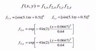
STALAGMITE FUNCTION-

STALAGMITE FUNCTION CODE:

function [F] = stalagmitee(input_vector)

x = input_vector(1);
y = input_vector(2) ; 

f1 = (sin(5.1*pi*x + 0.5))^6 ;
f2 = (sin(5.1*pi*y + 0.5))^6 ;
f3 = exp((-4*log(2)*((x-0.0667)^2/0.64))) ;
f4 = exp((-4*log(2)*((y-0.0667)^2/0.64))); 


F = f1*f2*f3*f4*-1;

end 

MAIN CODE:

clear all
close all
clc
 x = linspace(0,0.6,150);
 y = linspace(0,0.6,150);
 
 %converting 1D array into 2D array 
  [xx, yy] = meshgrid(x,y) ;
  iterations = 50 ;
  
  %stalagmitesimar function  
  for i = 1:length(xx)
      for j = 1:length(yy)
          input_vector(1) = xx(i,j);
          input_vector(2) = yy(i,j);
          f(i,j) = stalagmitee(input_vector);
      end
  end
  
%  1st iteration - studying the statistical behaviour
  
  tic
  for i = 1:iterations 
      [inputs,f_optimum(i)] = ga(@stalagmitee,2);
      x_optimum(i) = inputs(1) ;
      y_optimum(i) = inputs(2) ; 
  end
  iteration_1_time = toc
  
   %plotting
   
   figure(1)
   subplot(2,1,1)
   hold on 
   surfc(xx,yy,f)
   shading interp
   plot3(x_optimum,y_optimum,f_optimum,'marker','o','markersize',5,'markerfacecolor','r')
   title('unbouded inputs')
   subplot(2,1,2)
   plot(f_optimum)
   xlabel('Iterations')
   ylabel('Function maximum')
   
   %2nd iterations with upper and lower limits 
   
   tic 
   for i = 1:iterations
       [inputs , f_optimum(i)] = ga(@stalagmitee,2,[],[],[],[],[0;0],[1;1]);
       x_optimum(i) = inputs(1);
       y_optimum(i) = inputs(2);
   end
   
   iteration_2_time = toc 
   
   %plotting 
   figure(2)
   subplot(2,1,1)
   hold on
   surfc(xx,yy,f)
   shading interp
   plot3(x_optimum,y_optimum,f_optimum,'marker','o','markersize',5,'markerfacecolor','r')
   title('Bounded inputs')
   subplot(2,1,2)
   plot(f_optimum)
   xlabel('Iterations')
   ylabel('Function maximum')
   
   %3rd iteration - increasing the size f population
   
   options = optimoptions('ga');
   options = optimoptions(options,'populationsize',200)
   
   tic
   for i=1:iterations 
       [inputs, f_optimum(i)] = ga(@stalagmitee,2,[],[],[],[],[0;0],[0.2;0.2],[],[],options);
       x_optimum(i) = inputs(1);
       y_optimum(i) = inputs(2);
   end 
   
   iteration_3_time = toc 
   
   %plotting 
   figure(3)
   subplot(2,1,1)
   surfc(xx,yy,f)
   hold on
   shading interp
   plot3(x_optimum,y_optimum,f_optimum,'marker','o','markersize',5,'markerfacecolor','r')
   title('Bounded inputs with modified population size')
   hold off
   subplot(2,1,2)
   plot(f_optimum)
   xlabel('Iterations')
   ylabel('Function maximum')
    
    
    
   
   
   
    

EXPLANATION OF CODE:
(.) Initially ,the stalagmite function was mentioned with appropriate argument vectors.
(.)The progrma has been subdivided into three studies based on thre limitations of the previous study.
(.)First study deals with unbounded inputs ,thereby explaining the boundary wherein the results can be obtained.
(.)second study brings in thr aspect of bounded inputs providing a better solution for the drawback faced.
(.)Third study lays a appreciable platform to detemine the exact solution.
(.)Plots of all the three studies have been displayed , thus giving a clear insight of the results.

RESULT:

CASE1-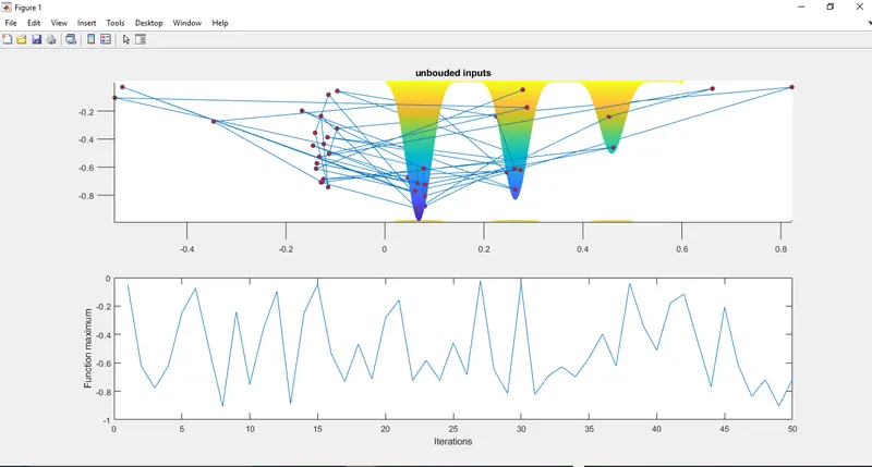

CASE2-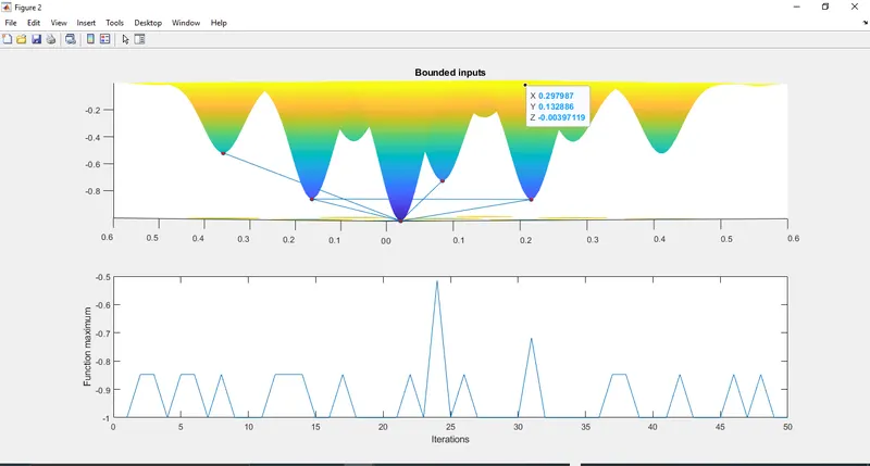

CASE3-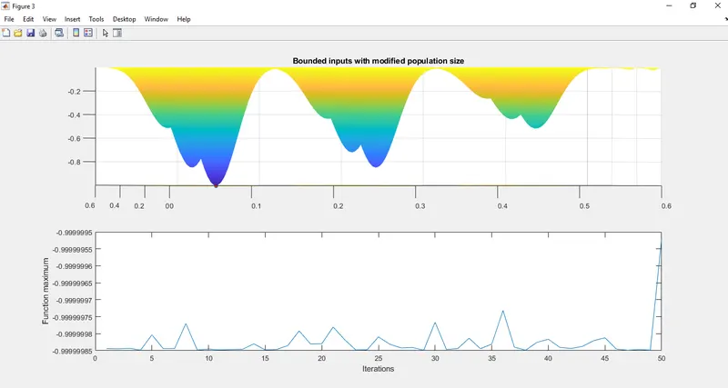

CONCLUSION: The Global Maxima is calculated by population sizing nd the plots provide a visual context of the solution and verifies the authenticity of the obtained value.