Week 4.1 - Genetic Algorithm

https://skill-lync.com/myprojects/edit/48012

Genetic Algorithm.- GA is one of the optimization algorithms which is based on natural selection. Genetic Algorithms(GAs) are adaptive heuristic search algorithms that belong to the larger part of evolutionary algorithms. The genetic algorithm (GA), developed by John Holland and his collaborators in the 1960s and 1970s (Holland, 1975; De Jong, 1975), is a model or abstraction of biological evolution based on Charles Darwin's theory of natural selection.

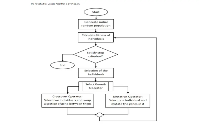
There are 4 major parts of genetic algorithms:-

1. The individual in population compete for resources and mate
2. Those individuals who are successful (fittest) then mate to create more offspring than others
3. Genes from “fittest” parents propagate throughout the generation, that is sometimes parents create offspring which are better than either parent.
4. Thus each successive generation is more suited for their environment

Genetic Algorithms works on these are important terminology:

1. Fitness score- Finding the best-suited solution for a given fitness function. The GAs maintains the population of n individuals (chromosome/solutions) along with their fitness scores. The individuals having better fitness scores are given more chances to reproduce than others.
2. Selection- The idea is to give the individuals a good fitness score and pass their genes to successive generations.
3. Cross-over-This represents mating between individuals. Two individuals are selected using a selection operator and crossover sites are chosen randomly. Then the genes at these crossover sites are exchanged thus creating a completely new individual (offspring).
4. Mutation- The key idea is to insert random genes in offspring to maintain the diversity in the population to avoid premature convergence.

The working principle of the genetic algorithm is given below

1) Randomly initialize populations p

2) Determine fitness of the population

3) Until convergence repeat:

1. a) Select parents from population
2. b) Crossover and generate a new population
3. c) Perform mutation on new population
4. d) Calculate fitness for new population

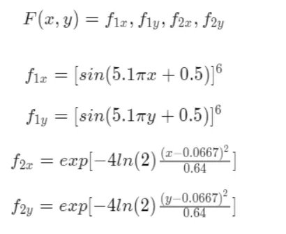
Stalagmite function:-A stalagmite function generally refers to the function with which we generate values over a stalagmite kind of surface for finding out the local and global maxima and minima of that particular function.

There is an inbuilt function in MATLAB for genetic algorithms. The syntax for the algorithm is given below.

• x = ga(fun,nvars) finds a local unconstrained minimum, x, to the objective function, fun. nvars is the dimension (number of design variables) of fun.

• x = ga(fun,nvars, A,b) finds a local minimum x to fun, subject to the linear inequalities A*x ≤ b. ga evaluates the matrix product A*x as if x is transposed (A*x')

.

• x = ga(fun,nvars,A,b,Aeq,beq) finds a local minimum x to fun, subject to the linear equalities Aeq*x = beq and A*x ≤ b. (Set A=[] and b=[] if no linear inequalities exist.) ga evaluates the matrix product Aeq*x as if x is transposed (Aeq*x').

• x = ga(fun,nvars,A,b,Aeq,beq,lb,ub) defines a set of lower and upper bounds on the design variables, x, so that a solution is found in the range lb ≤ x ≤ ub. (Set Aeq=[] and beq=[] if no linear equalities exist.)

• x = ga(fun,nvars,A,b,Aeq,beq,lb,ub,nonlcon) subjects the minimization to the constraints defined in nonlcon. The function nonlcon accepts x and returns vectors C and Ceq, representing the nonlinear inequalities and equalities respectively. ga minimizes the fun such that C(x) ≤ 0 and Ceq(x) = 0. (Set lb=[] and ub=[] if no bounds exist.)

• x = ga(fun,nvars,A,b,Aeq,beq,lb,ub,nonlcon,options) minimizes with the default optimization parameters replaced by values in options. (Set nonlcon=[] if no nonlinear constraints exist.) Create options using optimoptions.

• x = ga(fun,nvars,A,b,[],[],lb,ub,nonlcon,IntCon) or x = ga(fun,nvars,A,b,[],[],lb,ub,nonlcon,IntCon,options) requires that the variables listed in IntCon take integer values.

Explanation of code:-

• Creating two 1-D arrays stores in x and y variables.
• Generating 2-D array from given x and y using meshgrid command.
• For defining input for the stalagmite function,for loop used to the length of xx and yy with I and j variables to get the input vector for the function.
• The stalagmite function is defined using the given mathematical function, where the negative sign is used to convert minima to maxima.
• After preparing the inputs needed for the function, next step is to obtain the resultsfor 3 cases of the genetic algorithm. In first:ase or study, the maximum value of function is found out with no restrictions, no bounds and no limits.
• ga syntax to give values for inputs and optimum max value. The stalagmite function is called in 'ga syntax and number of variables 'nvars' are 2.
• To know the time that istaken to solve the loop for 50 iterations, 'tic' and 'toc'command is used before and after the loop respectively.
• Then the function created in the loop is plotted by using'surfc' command for 'xx, yy and function output'. To neglect the gridlines on the
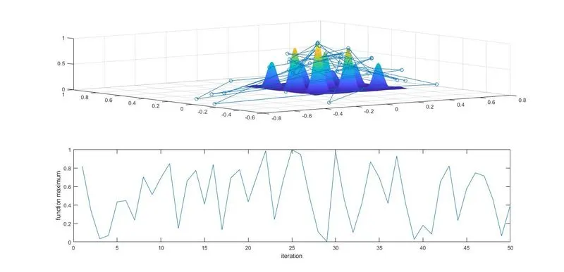
  surface and obtain a smooth and dean plot, 'shading interp' command is used. The 'subplot{2,1,1)' is used to plot multiple plots en same figure which also divides figure in grid of 2x1 and axes to be placed at 1.
• The 'plot3'command plots the 30 pointsat 'xopt, yopt and optimum value of function' with 'o shaped and red colour. The labels and title are
  then provided. Now in the same figure,the values of optimum function 'fopt' are plotted for 50 iterations.
• The results of the above case will be different for each time we run the program. To get same value each time, we need to restrict the program within specific bounds namely upper bound and lower bound. Theprocedu re for coding and plottind thisprocedu re issame as Study 1.The only diff erence is in the 'ga' syntax. Thistime the algorithm is provided lower limitsand upper limitsas [O;O]and [1;1] respectively.
• After plotting the resultsfor Study 2 or the bounded case, it is observed that theresults are not same every time the program tErminates. A solution to thisproblem isto increase the number of cases or iterations.
• Sofor Study 3, the number of iterations are increased to 300. So for this study,the syntax, "options o
  optimoptions('SolverName7Name7Value')" isused which returns with named parameter 'Populations' with the altered values '300'.
• The syntax for 'ga' contains'option' term and the rest of the code is same as for Study 1 and 2.

close all
clc
clear all;
x=linspace(0,0.6,150);
y=linspace(0,0.6,150);
num_spaces=50;
[xx,yy]=meshgrid(x,y);

for i = 1:length(xx)
for j= 1:length(yy)
input_vector(1)=xx(i,j);
input_vector(2)=yy(i,j);
f(i,j)=stalagmite(input_vector);
end
end
%type 1= unbound or stastical behaviour
tic
for i=1:num_spaces
[results,fopt(i)]=ga(@stalagmite,2)
xopt(i)=results(1)
yopt(i)=results(2)
end

study_time1=toc
figure(1)
subplot(2,1,1)
surf(x,y,-f)
shading interp
hold on
plot3(xopt,yopt,-fopt,'marker','o')
subplot(2,1,2)
plot(-fopt)
xlabel('iteration')
ylabel('function maximum')

%type 2= bounding the variable
tic
for i=1:num_spaces
[results,fopt(i)]=ga(@stalagmite,2,[],[],[],[],[0;0],[0.6;0.6])

% x = ga(fun,nvars,A,b,Aeq,beq,lb,ub,nonlcon) subjects the minimization to the constraints defined in nonlcon. The function nonlcon accepts x and returns vectors C and Ceq, representing the nonlinear inequalities and equalities respectively. ga minimizes the fun such that C(x) ≤ 0 and Ceq(x) = 0. (Set lb=[] and ub=[] if no bounds exist.)

xopt(i)=results(1)
yopt(i)=results(2)
end

study_time2=toc
figure(2)
subplot(2,1,1)
surf(x,y,-f)
shading interp
hold on
plot3(xopt,yopt,-fopt,'marker','o')
subplot(2,1,2)
plot(-fopt)
xlabel('iteration')
ylabel('function maximum')

%type 3 incresed initial population
tic
options=optimoptions('ga')
options=optimoptions(options,'populationsize',500)
for i=1:num_spaces
[results,fopt(i)]=ga(@stalagmite,2,[],[],[],[],[0;0],[0.6;0.6])
xopt(i)=results(1)
yopt(i)=results(2)
end

study_time3=toc
figure(3)
subplot(2,1,1)
surf(x,y,-f)
shading interp
hold on
plot3(xopt,yopt,-fopt,'marker','o')
subplot(2,1,2)
plot(-fopt)
xlabel('iteration')
ylabel('function maximum')

Figure 1 for stastical behaviour

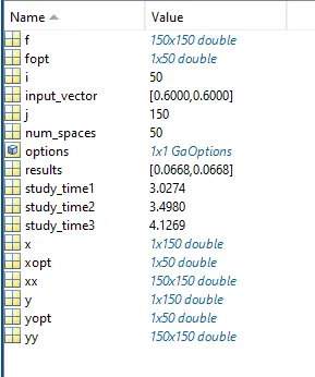
2 Bound to given value of x and y

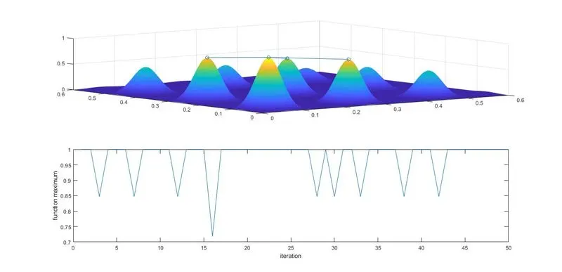
# result to get optimal in every iteration incrsed the population size .

https://in.mathworks.com/help/gads/example-global-vs-local-minima-with-ga.html

https://in.mathworks.com/help/gads/ga.html

https://www.geeksforgeeks.org/genetic-algorithms/