Curve Fitting

Curve fitting examines the relationship between one or more predictors (independent variables) and a response variable (dependent variable), intending to define a "best fit" model of the relationship. The curve fit is the process of constructing a curve or mathematical function, that has the best fit to a series of data points, possibly subject to constraints. Curve fitting can involve either interpolation. Where an exact fit to the data is required. Or smoothing, in which a ‘smooth’ function is constructed that approximately fit the data. Fitted curves can aid data visualization, infer values of a function where no data are available, and summarize the relationships among two or more variables.

To find the best fit for the curve, depends upon the degree of the polynomials. Some functions help us to find the accuracy of the fitted curves, those parameters are given below:

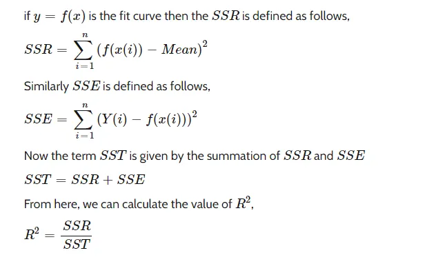
R-square value:- R-square is the square of the correlation between the actual value and predicted value. It ranges from 0 to 1. 1 is the best fit and 0 will be the worse fit. R- square is defined as the ratio of the sum of the squares of the regressions(SSR) and the total sum of the squares(SST). Where SST is defined as the sum of the squares of the regressions(SSR) and the square difference between actual data and predicted data(SSE).

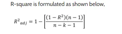
Adjusted R- value- The adjusted R-squared is a modified version of R-squared that accounts for predictors that are not significant in a regression model. In other words, the adjusted R-squared shows whether adding additional predictors improves a regression model or not. To understand adjusted R-squared, an understanding of R-squared is required.

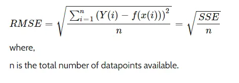
Root mean square value- The root-mean-square deviation (RMSD) or root-mean-square error (RMSE) is a frequently used measure of the differences between values (sample or population values) predicted by a model or an estimator and the values observed.

Stepwise explanation

1. Start the program with close all and clear all
2. Load the data of cp vs temperature using the load function
3. Assign the loaded data as cp_data variables.
4. 1st column of data assigned to the t variables.
5. 2nd column of data assigned to the cp variables.
6. To find the coefficient of the polynomial function we use polyfit command in which it returns the coefficients for a polynomial p(x) of degree n that is the best fit for the data in y.

coefficient=polyfit(x,y,n) in which x is temperature, y is cp, and n is the degree of the polynomial.

1. To predict the value of cp we use polyval command in which coefficient and x(temperature data) will be used as input.
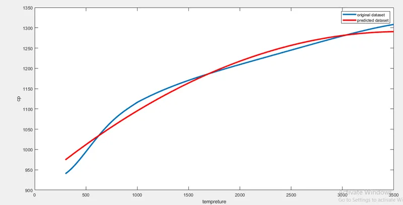
2. To compare the predicted value and original value we use the plot command.
3. Plotting the predicted and actual value in which y label as cp and x label as cp.
4. To check the correctness of the plotted curved fitting
5. SSE and SSR are calculated using for loop
6. SST is calculated using SSE and SSR
7. R squared and RMSE is calculated using SSR and SST.

Code:-

clear all;
close all;
clc

cp_data=load('data');
tempreture=cp_data(:,1);
cp=cp_data(:,2);

%plot

plot(tempreture,cp,'linewidth',3)
xlabel('tempreture')
ylabel('cp')
hold on
%curve Fit

co_effect=polyfit(tempreture,cp,1)
predicted_cp=polyval(co_effect,tempreture);
plot(tempreture,predicted_cp,'linewidth',3,'color','r')
legend('original dataset','predicted dataset');

%error estimation

add=0;
for i=1:3200
add=add+cp_data(i,2);
end

mean=add/3200;

ssr=0;
sse=0;

for j=1:3200
ssr=ssr+(predicted_cp(j)-mean)^2;
sse=sse+(cp_data(j,2)-predicted_cp(j))^2

end

sst=ssr+sse
r_square=ssr/sst

In Split wise

1. Start the program with close all and clear all
2. Load the data of cp vs temperature using the load function
3. Assign the loaded data as cp_data variables.
4. 1st column of data assigned to the t variables.
5. 2nd column of data assigned to the cp variables.
6. Divide the cp and temperature into four equal subparts. Perform the step on each subpart of temperature and cp.

1. To find the coefficient of the polynomial function we use polyfit command in which it returns the coefficients for a polynomial p(x) of degree n that is the best fit for the data in y.
2. coefficient=polyfit(x,y,n) in which x is temperature, y is cp, and n is the degree of the polynomial.
3. To predict the value of cp we use polyval command in which coefficient and x(temperature data) will be used as input.
4. To check the correctness of the plotted curved fitting
5. SSE and SSR are calculated using for loop
6. SST is calculated using SSE and SSR
7. R squared and RMSE is calculated using SSR and SST.

7. . Averaging all RMSE and R_squared values.
8. Plotting the all predicted value and original value.

Code:-

clear all;
close all;
clc;

cp_data=load('data')
t=cp_data(:,1);
t1=t(1:800);
t2=t(801:1600);
t3=t(1601:2400);
t4=t(2401:3200);
cp=cp_data(:,2);
cp1=cp(1:800)
cp2=cp(801:1600);
cp3=cp(1601:2400);
cp4=cp(2401:3200);

%first set

[coef_1,S1,mu1]=polyfit(t1,cp1,3);
pred_cp1=polyval(coef_1,t1,S1,mu1);

for i=1:length(cp1);
x1(i)=(pred_cp1(i)-cp1(i))^2;
y1(i)=(pred_cp1(i)-mean(cp1))^2;
end

SSE_1=sum(x1);
SSR_1=sum(y1);
R_sq_1=(SSR_1/(SSE_1+SSR_1));
RMSE_1=(SSE_1/length(t1))^0.5;

%2nd Set

[coef_2,s2,mu2]=polyfit(t2,cp2,3);
pred_cp2=polyval(coef_2,t2,s2,mu2);

for i=1:length(cp2);
x2(i)=(pred_cp2(i)-cp2(i))^2;
y2(i)=(pred_cp2(i)-mean(cp2))^2;
end

SSE_2=sum(x2);
SSR_2=sum(y2);
R_sq_2=(SSR_2/(SSE_2+SSR_2));
RMSE_2=(SSE_1/length(t2))^0.5;

%3rd set

[coef_3,s3,mu3]=polyfit(t3,cp3,3);
pred_cp3=polyval(coef_3,t3,s3,mu3);

for i=1:length(cp3);
x3(i)=(pred_cp3(i)-cp3(i))^2;
y3(i)=(pred_cp3(i)-mean(cp3))^2;
end

SSE_3=sum(x3);
SSR_3=sum(y3);
R_sq_3=(SSR_3/(SSE_3+SSR_3));
RMSE_3=(SSE_3/length(t3))^0.5;

%4th set

[coef_4,s4,mu4]=polyfit(t4,cp4,3);
pred_cp4=polyval(coef_4,t4,s4,mu4);

for i=1:length(cp4);
x4(i)=(pred_cp4(i)-cp4(i))^2;
y4(i)=(pred_cp4(i)-mean(cp4))^2;
end

SSE_4=sum(x4);
SSR_4=sum(y4);
R_sq_4=(SSR_4/(SSE_4+SSR_4));
RMSE_4=(SSE_4/length(t4))^0.5;

R_sq_total=(R_sq_1+R_sq_2+R_sq_3+R_sq_4)/4;
RMSE_total=(RMSE_1+RMSE_2+RMSE_3+RMSE_4)/4;

%Ploting

plot(t,cp,'linewidth',4,'color','b')
hold on
plot(t1,pred_cp1,'linewidth',3,'color','y')
hold on
plot(t2,pred_cp2,'linewidth',3,'color','g')
hold on
plot(t3,pred_cp3,'linewidth',3,'color','m')
hold on
plot(t4,pred_cp4,'linewidth',3,'color','r')
xlabel('Tempreture[K]');
ylabel('cp');
legend('original','first set','second set','3rd_set','4th_set');

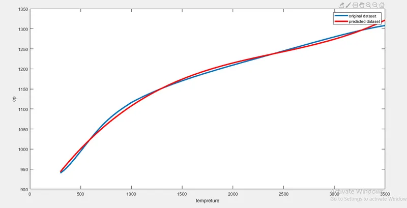
In MATLAB there is an inbuilt function of the curve fitting app.

1. Open the curve fitting app
2. Select the X data and Y data
3. We can select the degree of the polynomial.
4. Curve fit app automatically generates curve
5. We can increase the degree of the polynomial to get a perfect fit.

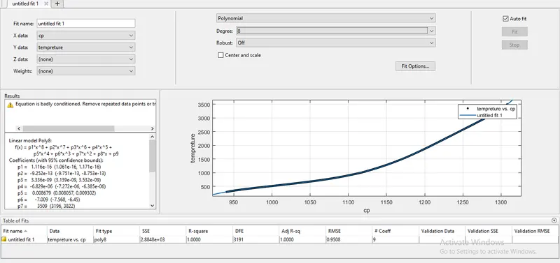
Best fit

For the best fit, the r_sqaured value will be 1. The curve fit app will be the best way to get the curve fitting.