Solve and create plot for Otto cycle in MATLAB

Objective- To write a code in MATLAB to solve and create plot for Otto cycle. The code should calculate the thermal efficiency of the engine and also should create a PV diagram of the otto cycle.

SOLUTION:

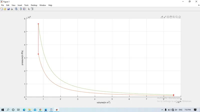
A Matlab code was written to solve the Otto cycle, to find the pressure, volume and tem perature values at the various state points. Further, the code generates a plot of the Otto cycle with respect to the i nput variables given and also calculates the thermal efficiency of the engine.

Explanation:

To write the code in MATLAB, first we have to understand the basic of the otto cycle. The otto cycle is an air standard cycle which consist of 4 thermodynamic process as follows:-

1---->2. isentropic compression

2----->3. isochoric compression (heat transfer)

3----->4. isentropic expansion

4----->1. isochoric expansion (heat transfer)

For ploting this process path , the engine kinematics will be used. for engine kinematics we assumed some engine geometric parameters such as

Bore=0.1m

Con_rod length=0.1m

compression ratio=12

Gamma=1.4

from this we calculated the swept volume and clearance volume which are function of these variables.

For calculating process pathm, the basic input parameters are assumed for genrating plot

Pressure at stage 1(p1)= 101325 pa

tempreture at stage 1 (t1)=500K

tempreture at stage 3 (t3)=2300K

Remaining stage parameters are calculated using ideal gas equation

(PV^Y)a = (PV^Y)a

(PV/T)a = (PV/T)b

Volumetric_expansion and Volumetric_compression are calculated using below formula

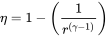
The thermal efficiency of the otto cycle is calculated

Error faced in the ploting the process path. by revising the concept of ploting the line in matlab able to overcome the error.

Outputs generated :
1. All values found at the state points was printed as a table
⦁ The otto cycle plot was generated
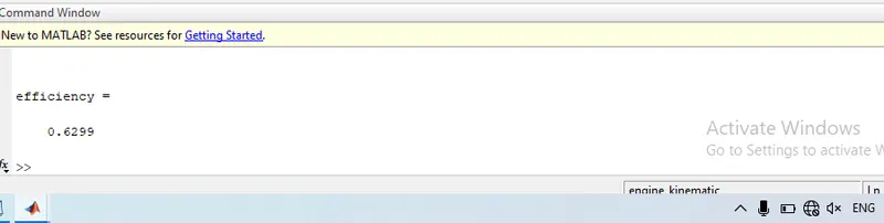
⦁ The efficiency of the cycle was calculated and printed

MATLAB code

clear all
close all
clc

%static variables
p1=101325;
t1=500;
t3=2300;
gamma=1.4;
crank_start=0;
crank_end=180;

%Engine geometric parameters
bore=0.1;
stroke=0.1;
con_rod=0.15;
cr=12;

%Calculating the swept volume and the clearnce volume
v_swept=(pi/4)*bore^2*stroke;
v_clerance=v_swept/(cr-1);

v1=v_swept+v_clerance;
v2=v_clerance;

%state variables at state point 2
% p2v2^gamma=p1v1^gamma
%p2=p1*(v1/v2)^gamma

p2=p1*cr^gamma;

%p1*v1/t1=p2*v2/t2;
t2=(p2/p1)*(v2/v1)*t1;

constant_c=p1*v1^gamma;
v_compression=engine_kinematic(bore,stroke,con_rod,cr,crank_start,crank_end);
P_compression=constant_c./v_compression.^gamma;

%state variables at state point 3
%p2*v2/t2=p3*v3/t3;

v3=v2;
p3=p2*t3/t2;

constant_c=p3*v3^gamma;
v_expansion=engine_kinematic(bore,stroke,con_rod,cr,180,0);
P_expansion=constant_c./v_expansion.^gamma;

%state variables at state 4;
%p3*v3^gamma=p4*v4^gamma;

v4=v1;
p4=p3*(v3/v4)^gamma;

%thermal efficiency
efficiency= 1-1/cr^(gamma-1)

figure(1)
hold on
plot(v1,p1,'*','color','r')
plot(v_compression,P_compression)
plot(v2,p2,'*','color','r')
plot(v3,p3,'*','color','r')
plot(v_expansion,P_expansion)
plot(v4,p4,'*','color','r')
plot([v2 v3],[p2 p3],'color','r')
plot([v4 v1],[p4 p1],'color','r')

xlabel('volume(in m^3)')
ylabel('pressure(in Pa)')
grid on

Code for calling engine_kinematic function

function[v]=engine_kinematic(bore,stroke,con_rod,cr,crank_start,crank_end)
%Engine geometric parameters

a=stroke/2;
R=con_rod/a;

%Calculating the swept volume and the clearnce volume
v_s=(pi/4)*bore^2*stroke;
v_c=v_s/(cr-1)

theta=linspace(crank_start,crank_end,100);
term1=0.5*(cr-1);
term2=R+1-cosd(theta);
term3=(R^2-sind(theta).^2).^0.5;

v= (1+term1*(term2-term3)).*v_c;

end