Week 4.1 - Genetic Algorithm

Ans:

Genetic Algorithm:

• A genetic algorithm (GA) is a method for solving both constrained and unconstrained optimization problems based on a natural selection process that mimics biological evolution.
• The genetic algorithm (GA), developed by John Holland and his collaborators in the 1960s and 1970s, is a model or abstraction of biological evolution based on Charles Darwin's theory of natural selection.
• Genetic algorithms are randomized search algorithms that have been developed in an effort to imitate the mechanics of natural selection and natural genetics.
• Genetic algorithms operate on string structures, like biological structures, which are evolving in time according to the rule of survival of the fittest by using a randomized yet structured information exchange. Thus, in every generation, a new set of strings is created, using parts of the fittest members of the old set. The main characteristics of a genetic algorithm are as follows:

1. The genetic algorithm works with a coding of the parameter set, not the parameters themselves.
2. The genetic algorithm initiates its search from a population of points, not a single point.
3. The genetic algorithm uses payoff information, not derivatives.
4. The genetic algorithm uses probabilistic transition rules, not deterministic ones.

Flow Chart:

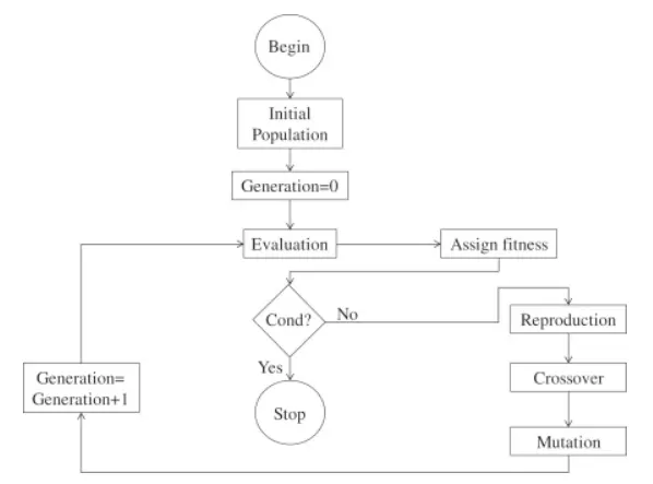
Step-1: Initialization.

Step-2: Select Parents & perform crossover.

Step-3: Mutate offsprings.

Step-4: Merge main population and offsprings.

Step-5: Evaluate, sort and select.

Step-6: Go to Step-2, if it is needed.

Stalagmite Function: It is a mathematical model which helps us generate local minimas and maximas. It is a 3D function.

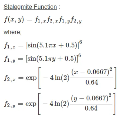
Stalagmite Function Code: (stalagmite.m)

function [fun]=stalagmite(input_vector)
x=input_vector(1);
y=input_vector(2);

f1x=[sin(5.1*pi.*x+0.5)]^6;
f1y=[sin(5.1*pi.*y+0.5)]^6;
    
f2x=exp(-4*log(2).*((x-0.0667).^2)/0.64);
f2y=exp(-4*log(2).*((y-0.0667).^2)/0.64);

fun=-(f1x*f1y*f2x*f2y);
end

get_stalagmite.m function code:

function[f]=get_stalagmite(x,y)
[xx,yy]=meshgrid(x,y);

for i=1:length(xx)
    for j=1:length(yy)
        input_vector(1)=xx(i,j);
        input_vector(2)=yy(i,j);
        f(i,j)=stalagmite(input_vector);
    end
end
end

Explanation: The above code generates the stalagmite 3D surface using meshgrid command. The point xx and yy are used to create 2D array and this is used to input in the stalagmite function using two for loops within which it is automatically called when the get_stalagmite functuon is initiated.

MATLAB Code to optimise the stalagmite function and find the global maxima of the function:

%Write a code in MATLAB to optimise the stalagmite function and find the global maxima of the function.
%Genetic Algorithm code
clear all;
close all;
clc;

%defining our search space
x=linspace(0,0.6,150);
y=linspace(0,0.6,150);

%run the Genetic algorithm 60 times
num_cases=50;

%calls the get_stalagmite.m function which generates the stalagmite 3D
%surface using meshgrid, where point xx & yy are used to create 2D array
%and this is used to input in the stalagmite function using two for loops
%within which it is automatically called when the get_stalagmite function
%is initiated
f=get_stalagmite(x,y);

%Study-1 : Statistical behavior without bounds
tic %evaluation time starts
for i=1:num_cases
    [inputs,fopt(i)]=ga(@stalagmite,2);
    xopt(i)=inputs(1);
    yopt(i)=inputs(2);
end
study1_time=toc; %evaluation time stops

figure(1)
subplot(2,1,1)
hold on
surfc(x,y,-f)
xlabel('x-axis');ylabel('y-axis');zlabel('z-axis');
shading interp
plot3(xopt,yopt,-(fopt),'marker','o','markersize',5,'markerfacecolor','r')
title('Unbounded Inputs');

subplot(2,1,2)
plot(-fopt);
xlabel('Number of Iterations');
ylabel('Function Maximum');


%Study-2 : Statistical behavior with Upper & Lower bounds
tic %evaluation time starts
for i=1:num_cases
    [inputs,fopt(i)]=ga(@stalagmite,2,[],[],[],[],[0;0],[1;1]);
    xopt(i)=inputs(1);
    yopt(i)=inputs(2);
end
study2_time=toc; %evaluation time stops

figure(2)
subplot(2,1,1)
hold on
surfc(x,y,-f)
xlabel('x-axis');ylabel('y-axis');zlabel('z-axis');
shading interp
plot3(xopt,yopt,-(fopt),'marker','o','markersize',5,'markerfacecolor','r')
title('Bounded Inputs');

subplot(2,1,2)
plot(-fopt);
xlabel('Number of Iterations');
ylabel('Function Maximum');

%Study-3 : Statistical behavior with increase genetic algorithm iterations
options=optimoptions('ga');
options=optimoptions(options,'PopulationSize',170); %polulation size 170

tic %evaluation time starts
for i=1:num_cases
    [inputs,fopt(i)]=ga(@stalagmite,2,[],[],[],[],[0;0],[1;1],[],[],options);
    xopt(i)=inputs(1);
    yopt(i)=inputs(2);
end
study3_time=toc; %evaluation time stops

figure(3)
subplot(2,1,1)
hold on
surfc(x,y,-f)
xlabel('x-axis');ylabel('y-axis');zlabel('z-axis');
shading interp
plot3(xopt,yopt,-(fopt),'marker','o','markersize',5,'markerfacecolor','r')
title('Bounded Inputs with modified polulation size');

subplot(2,1,2)
plot(-fopt);
xlabel('Number of Iterations');
ylabel('Function Maximum');

OUTPUT PLOTS:

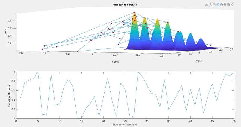
Figure-1: Statistical behavior of Unbounded Inputs

Evaluation Time:

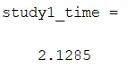
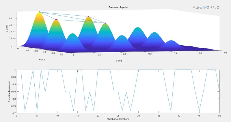
Figure-2: Statistical behavior of Bounded Inputs

Evaluation Time:

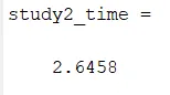
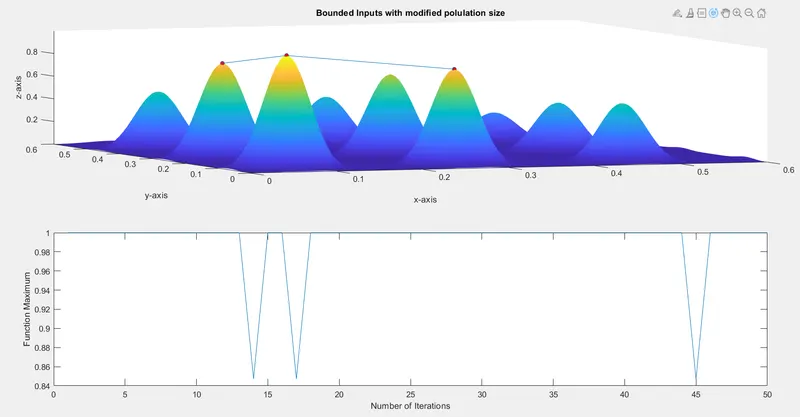
Figure-3: Statistical behavior of Bounded Inputs with modified population size

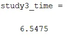
Evaluation Time:

Explantion of "ga" matlab command: (reference from help ga on command window)

ga Constrained optimization using genetic algorithm.
ga attempts to solve problems of the following forms:
min F(X) subject to: A*X <= B, Aeq*X = Beq (linear constraints)
X C(X) <= 0, Ceq(X) = 0 (nonlinear constraints)
LB <= X <= UB
X(i) integer, where i is in the index
vector INTCON (integer constraints)

Note: If INTCON is not empty, then no equality constraints are allowed.
That is:-
* Aeq and Beq must be empty
* Ceq returned from NONLCON must be empty

X = ga(FITNESSFCN,NVARS) finds a local unconstrained minimum X to the
FITNESSFCN using ga. NVARS is the dimension (number of design
variables) of the FITNESSFCN. FITNESSFCN accepts a vector X of size
1-by-NVARS, and returns a scalar evaluated at X.

X = ga(FITNESSFCN,NVARS,A,b) finds a local minimum X to the function
FITNESSFCN, subject to the linear inequalities A*X <= B. Linear
constraints are not satisfied when the PopulationType option is set to
'bitString' or 'custom'. See the documentation for details.

X = ga(FITNESSFCN,NVARS,A,b,Aeq,beq) finds a local minimum X to the
function FITNESSFCN, subject to the linear equalities Aeq*X = beq as
well as A*X <= B. (Set A=[] and B=[] if no inequalities exist.) Linear
constraints are not satisfied when the PopulationType option is set to
'bitString' or 'custom'. See the documentation for details.

X = ga(FITNESSFCN,NVARS,A,b,Aeq,beq,lb,ub) defines a set of lower and
upper bounds on the design variables, X, so that a solution is found in
the range lb <= X <= ub. Use empty matrices for lb and ub if no bounds
exist. Set lb(i) = -Inf if X(i) is unbounded below; set ub(i) = Inf if
X(i) is unbounded above. Linear constraints are not satisfied when the
PopulationType option is set to 'bitString' or 'custom'. See the
documentation for details.

X = ga(FITNESSFCN,NVARS,A,b,Aeq,beq,lb,ub,NONLCON) subjects the
minimization to the constraints defined in NONLCON. The function
NONLCON accepts X and returns the vectors C and Ceq, representing the
nonlinear inequalities and equalities respectively. ga minimizes
FITNESSFCN such that C(X)<=0 and Ceq(X)=0. (Set lb=[] and/or ub=[] if
no bounds exist.) Nonlinear constraints are not satisfied when the
PopulationType option is set to 'bitString' or 'custom'. See the
documentation for details.

X = ga(FITNESSFCN,NVARS,A,b,Aeq,beq,lb,ub,NONLCON,options) minimizes
with the default optimization parameters replaced by values in OPTIONS.
OPTIONS can be created with the OPTIMOPTIONS function. See OPTIMOPTIONS
for details. For a list of options accepted by ga refer to the
documentation.

X = ga(FITNESSFCN,NVARS,A,b,[],[],lb,ub,NONLCON,INTCON) requires that
the variables listed in INTCON take integer values. Note that ga does
not solve problems with integer and equality constraints. Pass empty
matrices for the Aeq and beq inputs if INTCON is not empty.

X = ga(FITNESSFCN,NVARS,A,b,[],[],lb,ub,NONLCON,INTCON,options)
minimizes with integer constraints and the default optimization
parameters replaced by values in OPTIONS. OPTIONS can be created with
the OPTIMOPTIONS function. See OPTIMOPTIONS for details.

CONCLUSIONS:

• If we compare the evaluation time for the statistical behavior of Unbounded inputs, Bounded inputs & Bounded inputs with modified population size, then the study time for the bounded inputs with modified polulation size is more than the other two, however it provides the optimum solution (figure-3) than figure-1 & 2.
• Furthermore, we can optimize the problem by modifying the polulation sizes to obtain the global maxima.