Week 3 - Solving second order ODEs

Ans:

Objective: Write a program that solves the following ODE. This ODE represents the equation of motion of a simple pendulum with damping.

............equation(i)

where;

g = gravity in m/s2,

L = length of the pendulum in m,

m = mass of the ball in kg,

b=damping coefficient.

Given Input parameters:

L=1 metre,

m=1 kg,

b=0.05.

g=9.81 m/s2.

Requirement:

To simulate the pendulum motion between 0-20 sec, for angular displacement=0,angular velocity=3 rad/sec at time t=0.

FUNCTION CODE:- (ode_function.m)

function[dtheta_dt]=ode_function(t,theta,b,g,l,m)
theta1=theta(1);
theta2=theta(2);
dtheta1_dt=theta2;
dtheta2_dt=-(b/m)*theta2-(g/l)*sin(theta1);
dtheta_dt=[dtheta1_dt;dtheta2_dt];
end

Explanation:

• The above function is created to convert the second order ODE into two first order ODEs such as dtheta1/dt=theta2 and dtheta2/dt=-(b/m)*theta2-(g/l)*sin(theta1).
• The value of the input argument of the function such that t,theta,b,g,l,m will be given as input in the main program and it will be executed during the function call.
• The output argument of the function is stored in dtheta_dt variable.

MAIN PROGRAM:- (pendulum_motion_animation.m)

%write a program that solves the following ODE. This ODE represents the equation of motion of a simple pendulum with damping
clear all;
close all;
clc;

% Given inputs
l=1; %length=1m
m=1; %mass=1kg
b=0.05; %damping coefficients
g=9.81; %gravity in m/s^2

%initial conditions
theta_0=[0;3]; %for angular displacement=0,angular velocity=3 rad/sec at time t=0sec

%Time Span
t_span=linspace(0,20,500); %Simulate the motion between 0-20 sec divided into 500 values

%Solving ODE using ode45 solver and calling the function ode_function.m
[t,results]=ode45(@(t,theta)ode_function(t,theta,b,g,l,m),t_span,theta_0);

%plotting
figure(1)
plot(t,results(:,1))
hold on
plot(t,results(:,2))
xlabel('Time')
ylabel('Angular Displacement & Angular Velocity')
grid on;
legend('Angular Displacement','Angular Velocity')
hold off

%plotting the animated motion of the pendulum
figure(2)
ct=1; %frame counter value
for i=1:length(t_span)
    %Considering one end of the position is fixed
    %initialize x_fixed_end=0, y_fixed_end=0;
    x_fixed_end=0;
    y_fixed_end=0;
    
    %calculate the moving end of the pendulum
    x_moving_end=l*sin(results(i,1));
    y_moving_end=-l*cos(results(i,1));
    
    %plot the animation
    plot([x_fixed_end x_moving_end],[y_fixed_end y_moving_end],[-0.5 0.5],[0 0],'linewidth',3)
    hold on
    plot(x_moving_end,y_moving_end,'marker','o','markerSize',30,'markerFacecolor','m')
    axis([-1.5 1.5 -1.5 1.5])
    xlabel('x-axis');
    ylabel('y-axis');
    title('MOTION OF PENDULUM');
    grid on
    pause(0.01)
    hold off
    M(ct)=getframe(gcf);
    ct=ct+1;
end
movie(M)
videofile=VideoWriter('ode_pendulum.avi','Uncompressed AVI');
open(videofile)
writeVideo(videofile,M)
close(videofile)


    

Explanation:

• The input parameters(b,g,l,m) have been initialized as per the given data.
• The initial condition is set for angular displacement=0,angular velocity=3 rad/sec at time t=0sec.
• The time points is considered in between 0-20 sec having 500 equally divided values using the linspace command.
• The ODE is solved using ode45 command which is an in-built solver and is a function of t and theta. Then the ode_function() is called which also has the same no of input arguments as that of the function code.
• In ode45() command, we also provide the time span and initial conditions for angular displacement and angular velocity.
• The outputs of the ODE is stored in results which is a (500x2) matrix, in which the first column represents the angular displacement and second column represents the angular velocity.
• Then, the output plot is plotted between the angular displacement and angular velocity vs time as shown in figure-1.
• To plot the animation of the pedulum motion, we have considered the initial starting position of the pendulum is fixed and assumed the co-ordinate (0,0). The moving end of the pendulum is calculated using the formulae given in the main code. For loop is used to update the pendulum position in each iterations till the time span size mentioned in the main code.
• The animation of the moving pendulum is created using the getframe command and storing the output value in an array called 'M'.
• A marker 'o' is considered with markersize of 30 to resemble like the pendulum ball.
• Movie of the array M is created using movie() command and the video is created and saved using VideoWriter command. The animated video is then opened and closed using open() and close() commands respectively.

OUTPUT PLOTS:

Figure-1: (Time vs Angular Displacement & Angular Velocity)

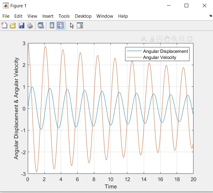
In the above plot, the displacement starts from 0 whereas the velocity starts from 3.

Figure-2: (Animated motion of Pendulum)

• Google Drive Link:

https://drive.google.com/file/d/17WK2sU6Htgzuo1b62HC7HkIpZ0v4pfq6/view?usp=sharing

• You Tube Video Link:

https://youtu.be/W-Be52PMk8A

RESULTS:

Successfully simulated and plotted the time vs angular displacement and angular velocity and also created the animated motion of the simple pendulum.