Week 4.1 - Genetic Algorithm
AIM- TO STUDY ABOUT CONCEPT OF GENETIC ALGORITHM AND CODE IN MATLAB TO OPTIMISE THE STALAGMITE FUNCTION AND CALCULATE THE GLOBAL MAXIMA OF THE FUNCTION
OBJECTIVE:-
- Write a code in MATLAB to optimise the stalagmite function and find the global maxima of the function.
- study of the concept of genetic algorithm and use the syntax for ga in MATLAB.
- Plot graphs for all 3 studies and for F maximum vs no. of iterations. Title and axes labels are a must, legends could be shown if necessary.
Genetic algorithm is process of natural selection where the fittest individuals are selected for reproduction in order to produce offspring of the next generation.
The process of natural selection starts with the selection of fittest individuals from a population. They produce offspring which inherit the characteristics of the parents and will be added to the next generation. If parents have better fitness, their offspring will be better than parents and have a better chance at surviving. This process keeps on iterating and at the end, a generation with the fittest individuals will be found.
This notion can be applied for a search problem. We consider a set of solutions for a problem and select the set of best ones out of them.
Five phases are considered in a genetic algorithm.
Initial population
Fitness function
Selection
Crossover
Mutation
ga
Find minimum of function using genetic algorithm
Description
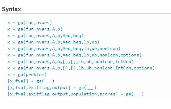
x = ga(fun,nvars)x, to the objective function, fun. nvars is the dimension (number of design variables) of fun.
Note
Passing Extra Parameters explains how to pass extra parameters to the objective function and nonlinear constraint functions, if necess
x = ga(fun,nvars,A,b)x to fun, subject to the linear inequalities A*x ≤ b. ga evaluates the matrix product A*x as if x is transposed (A*x')
x = ga(fun,nvars,A,b,Aeq,beq)x to fun, subject to the linear equalities Aeq*x = beq and A*x ≤ b. (Set A=[] and b=[] if no linear inequalities exist.) ga evaluates the matrix product Aeq*x as if x is transposed (Aeq*x').
x = ga(fun,nvars,A,b,Aeq,beq,lb,ub,nonlcon)nonlcon. The function nonlcon accepts x and returns vectors C and Ceq, representing the nonlinear inequalities and equalities respectively. ga minimizes the fun such that C(x) ≤ 0 and Ceq(x) = 0. (Set lb=[] and ub=[] if no bounds exist.)
x = ga(fun,nvars,A,b,[],[],lb,ub,nonlcon,IntCon)x = ga(fun,nvars,A,b,[],[],lb,ub,nonlcon,IntCon,options)IntCon take integer values.
Note
When there are integer constraints, ga does not accept linear or nonlinear equality constraints, only inequality constraints.
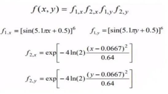
MAIN CODE
clear all
close all
clc
x = linspace(0,0.6,200);
y = linspace(0,0.6,200);
[xx yy] = meshgrid(x,y);
n=50;
%Study 1 - statistical model
for i = 1:length(xx)
 for j = 1:length(yy)

 input_vector(1) = xx(i,j);
 input_vector(2) = yy(i,j);

 f(i,j) = stalagmite(input_vector);

 end
end
figure(12)
surfc(xx,yy,-f)

xlabel('x value')
ylabel('y value')

shading interp
[inputs fval]=ga(@stalagmite,2);

tic
for i = 1:n

[inputs, fopt(i)] = ga(@stalagmite, 2);
xopt(i) = inputs(1);
yopt(i) = inputs(2);
end
figure(1)
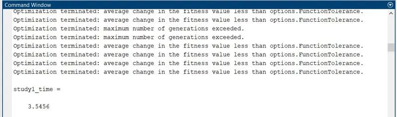
study1_time = toc
subplot(2,1,1)
surfc(x,y,f);
shading interp
hold on
plot3(xopt, yopt, fopt, 'b')
subplot(2,1,2)
plot(fopt)
xlabel('Optimal value')
ylabel('No. of iterations')
%Study 2 - Upper and lower bounds
tic
for i = 1:n

[inputs2, fopt2(i)] = ga(@stalagmite, 2, [], [], [], [], [0;0], [1;1]);
xopt2(i) = inputs2(1);
yopt2(i) = inputs2(2);
end
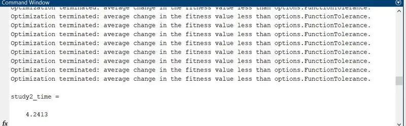
study2_time = toc
figure(2)
subplot(2,1,1)
surfc(x,y,f);
shading interp
hold on

plot3(xopt2, yopt2, fopt2, 'b' )
subplot(2,1,2)
plot(fopt2)
xlabel('No. of iterations')
ylabel('Optimum function')
%Study 3 - Setting a population size
options = optimoptions('ga', 'PopulationSize', 2000);
tic
for i = 1:n

[inputs3, fopt3(i)] = ga(@stalagmite, 2, [], [], [], [], [0;0], [1;1], [], [], options);
xopt3(i) = inputs3(1);
yopt3(i) = inputs3(2);
end
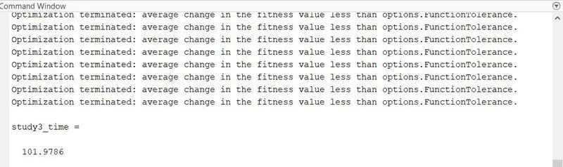
study3_time = toc
figure(3)
subplot(2,1,1)
surfc(x,y,f);
shading interp
hold on
plot3(xopt3, yopt3, fopt3, 'b')
subplot(2,1,2)
plot(fopt3)
xlabel('No. of iterations')
ylabel('Optimum function')
Initially two inputs are given namely x & y
using linspace command set the data b/w two number
meshgrid command used to cxreate of array of m*n mattrix
using for loop opration
the input vector stored the value of matrix xx & yy. output stored in f matrix after evaluated of stalagmite function
surf(x,y,z ) command used to create the 3-d diemenstional surface plot with a contour plot underneath.surface plot is a 3-diemensition suface that has solid edge colour& solid suface colour.
the label command is used axis of graph.
shading interp
hide the grid and graph smooth
% study 1 in genetic algorithm of random sampling
num_cases= 50 ie no,. of iteration in genetic algorithm
tic toc command is used calculate the time running.
% study 2 statistical behaviour in upper & lower bounds
% study 3 increasing the ga iteration
FUNCTION CODE
function [out] = stalagmite(input_vector)
%Defining input conditions
x=input_vector(1);
y=input_vector(2);
%Solving the equations to obtain the values of the function
f1x = (sin((5.1*pi*x)+0.5))^6;
f1y = (sin((5.1*pi*y)+0.5))^6;
f2x = exp(-4*log(2)*(((x-0.0667)^2)/0.64));
f2y = exp(-4*log(2)*(((y-0.0667)^2)/0.64));
F = f1x*f1y*f2x.*f2y;
%Output is set to negative in order to measure the global maxima instead of
%global minima %in the genetic algorithm

out = -F;
end
workspace:-
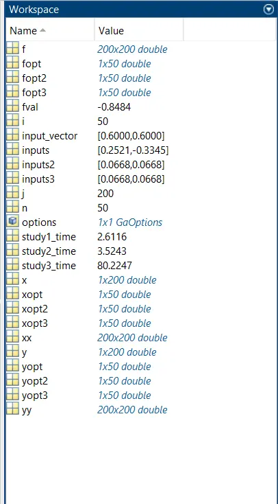
output:-