Week 4.1 - Genetic Algorithm

Aim

Write a code in MATLAB to optimise the stalagmite function and find the global maxima of the function

Theory

Optimization :

Optimization is the process of making something better. In any process, we have a set of inputs and a set of outputs as shown in the following figure.

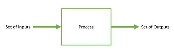
Optimization refers to finding the values of inputs in such a way that we get the best output values. The definition of best varies from problem to problem, but in mathematical terms, it refers to maximizing or minimizing one or more objective functions, by varying the input parameters. The set of all possible solutions or values which the inputs can take makes up the search space. In this search space, lies a point or a set of points which gives the optimal solution. The aim of optimization is to find that point or set of points in the search space.

Genetic Algorithm (GA) :

Genetic Algorithm (GA) is a search-based optimization technique based on the principles of Genetics and Natural Selection. It is frequently used to find optimal or near-optimal solutions to difficult problems which otherwise would take a lifetime to solve. It is frequently used to solve optimization problems, in research, and in machine learning. Nature has always been a great source of inspiration to all mankind. Genetic Algorithms (GAs) are search-based algorithms based on the concepts of natural selection and genetics. GAs are a subset of a much larger branch of computation known as Evolutionary Computation.

In GAs, we have a pool or a population of possible solutions to the given problem. These solutions then undergo recombination and mutation (like in natural genetics), producing new children, and the process is repeated over various generations. Each individual (or candidate solution) is assigned a fitness value (based on its objective function value) and the fitter individuals are given a higher chance to mate and yield more fitter individuals. This is in line with the Darwinian Theory of Survival of the Fittest. In this way, we keep evolving better individuals or solutions over generations, till we reach a stopping criterion.

Code Explanation

1. Search space is defined using linspace.
2. 2D mesh is created using meshgrid.

Syntax - [X,Y] = meshgrid(x,y)

3. Using the for loop stalagmite function is created for a very value of i&j.

4. surfc is used to make a 3D plot.

Syntax - surfc(X,Y,Z)

Genetic Algorithm GA

GA is used to optimize the stalagmite function by varying the inputs

Study 1

a. tic & toc is used to find the time duration of the function to execute.

b. For loop is used to check the condition of stalagmite function by different inputs of GA

Syntax - x=ga(fun, nvars)

fun - function

nvars - number of variables

c.subplot- Creating a figure with 2 stacked subplots

Syntax - subplot(m,n,p)

d. plots are made using the plot command

Study 2

Syntax for GA. - x=ga(fun, nvars, A, B, Aeq, Beq, lb, ub)

Study 3

Syntax for GA. - x=ga(fun, nvars, A, B, Aeq, Beq, lb, ub, nonlcon, intcon, options)

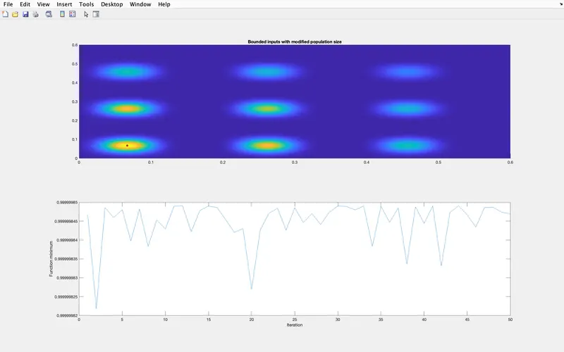
Here, we are using the population size 500 with the help of options to find the global maxima of the function.

Code

close all 
clear all
clc

% Defining our search space 
x = linspace(0,0.6,150);
y = linspace(0,0.6,150);
num_cases = 50 

% Creating a 2D Mesh
[xx yy] = meshgrid(x,y);

% Evaluating the Stalagmite Function

for i = 1 : length(xx)
    for j = 1 : length(yy)
        input_vector(1)=xx(i,j);
        input_vector(2)=yy(i,j);
        f(i,j) = stalagmite(input_vector);
    end
end

surfc(xx,yy,f)


 % Study 1 - Satistical behaviour  

 tic
 for i=1:num_cases
     [inputs, fopt(i)] = ga(@stalagmite, 2);
     xopt(i)=inputs(1);
     yopt(i)=inputs(2);
 end

fopt= -fopt;
time_study1=toc

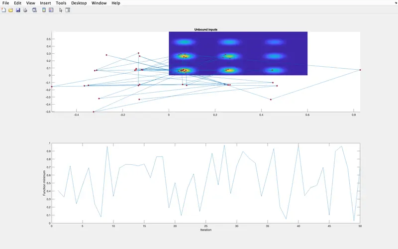
figure(1)
subplot(2,1,1)
hold on
surfc(x,y,-f)
shading interp
plot3(xopt,yopt,fopt,'marker','o','MarkerSize',5,'markerfacecolor','r')
title('Unbound inputs')
% Figure(2)
subplot(2,1,2)
plot(fopt)
xlabel('Iteration')
ylabel('Function minimum')


% Study 2 - Satistical behaviour with upper and lower bounds

 tic
 for i=1:num_cases
     [inputs2, fopt2(i)] = ga(@stalagmite,2,[],[],[],[],[0,0],[1,1]);
     xopt2(i)=inputs2(1);
     yopt2(i)=inputs2(2);
 end

fopt2= -fopt2;
time_study2=toc

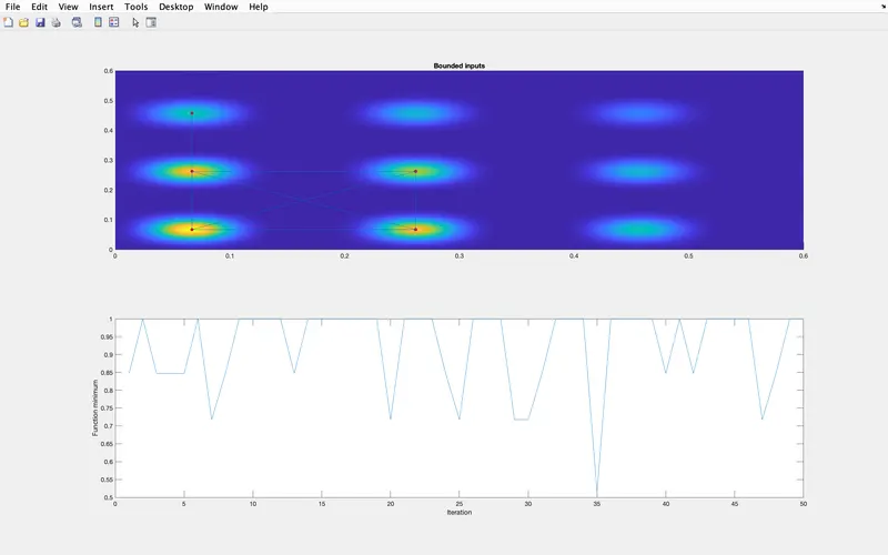
figure(2)
subplot(2,1,1)
hold on
surfc(x,y,-f)
shading interp
plot3(xopt2,yopt2,fopt2,'marker','o','MarkerSize',5,'markerfacecolor','r')
title('Bounded inputs')
% Figure(2)
subplot(2,1,2)
plot(fopt2)
xlabel('Iteration')
ylabel('Function minimum')


% Study 3 - Maximizing the population size to optimize the result

options = optimoptions('ga')
options = optimoptions(options,'PopulationSize',500);

 tic
 for i=1:num_cases
     [inputs3, fopt3(i)] = ga(@stalagmite,2,[],[],[],[],[0,0],[0.6,0.6],[],[],options);
     xopt3(i)=inputs3(1);
     yopt3(i)=inputs3(2);
 end
fopt3= -fopt3;
time_study3=toc

figure(3)
subplot(2,1,1)
hold on
surfc(x,y,-f)
shading interp
plot3(xopt3,yopt3,fopt3,'marker','o','MarkerSize',5,'markerfacecolor','r')
title('Bounded inputs with modified population size')
% Figure(2)
subplot(2,1,2)
plot(fopt3)
xlabel('Iteration')
ylabel('Function minimum')

Result

1. Unbound Inputs

2. Bound Inputs

3. Bounded inputs with modified population size

Reference

https://towardsdatascience.com/introduction-to-genetic-algorithms-including-example-code-e396e98d8bf3

https://skill-lync.com/knowledgebase/genetic-algorithm-explained

https://www.tutorialspoint.com/genetic_algorithms/genetic_algorithms_introduction.htm