Week 4.1 - Genetic Algorithm

Aim:To study about Genetic Algorithm,global maxima of stalagmite function using MATLAB.

OBJECTIVE :

1)To study about Genetic Algorithm and Stalagmite function.

2)Optimise the stalagmite function and find the global maxima of the function in MATLAB.

3)To plot graphs on the studies done using Genetic Algorithm.

Genetic Algorithm:

Nature has always been a great source of inspiration to all mankind. Genetic Algorithms (GAs) are search based algorithms based on the concepts of natural selection and genetics. GAs are a subset of a much larger branch of computation known as Evolutionary Computation.GAs were developed by John Holland and his students and colleagues at the University of Michigan, most notably David E. Goldberg and has since been tried on various optimization problems with a high degree of success.In GAs, we have a pool or a population of possible solutions to the given problem. These solutions then undergo recombination and mutation (like in natural genetics), producing new children, and the process is repeated over various generations. Each individual (or candidate solution) is assigned a fitness value (based on its objective function value) and the fitter individuals are given a higher chance to mate and yield more “fitter” individuals. This is in line with the Darwinian Theory of “Survival of the Fittest”.In this way we keep “evolving” better individuals or solutions over generations, till we reach a stopping criterion.Genetic Algorithms are sufficiently randomized in nature, but they perform much better than random local search (in which we just try various random solutions, keeping track of the best so far), as they exploit historical information as well.

How do genetic algorithms work?

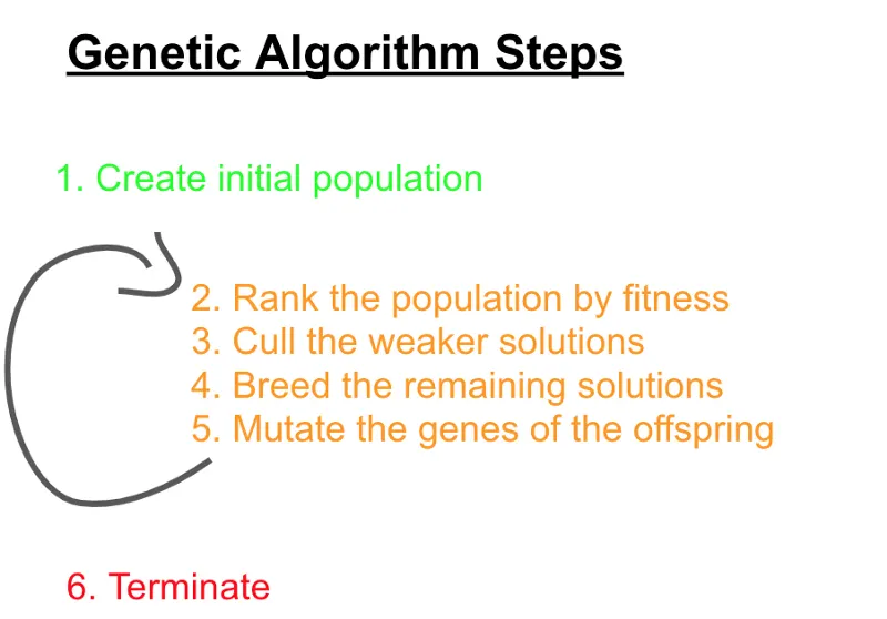
The basic steps in creating a genetic algorithm is as follows,

1. The algorithm creates a random initial population at beginning.
2. Then to create new population, the algorithm scores each member of the current population by computing its fitness value and converts them into a more usable range of values.
3. Then based on these new values the algorithm selects members, called as parents.
4. Then the algorithm produces children from the parents. Children are produced either by making random changes to a single parent which is mutation or by combining the vector entries of a pair of parents which is crossover.
5. In this way the algorithm replaces the current population with the children to form the next generation.
6. The algorithm stops when it reaches any one of the specified factors factors such as time limit, fitness limit, generations, function tolerance, constraint tolerance, etc.

The flowchart for Genetic Algorithm is given below,

Stalagmite function:

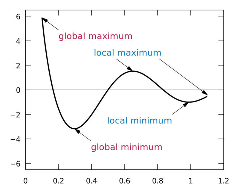
Stalagmite function is a mathematical model which helps to generate local minima and maxima. It is a three dimensional function and the way the function is designed is that it has a lot of local maxima or minima and one global maxima or minima. The name stalagmite is actually a type of rock formation that arises from the floor of a cave due to the accumulation of material deposited on the floor from ceiling drippings.

Syntax for Genetic Algorithm:

The ‘ga’ syntax in matlab is used to find the minimum of function using genetic algorithm.

• x = ga(fun,nvars,A,B,Aeq,Beq,lb,ub,nonlcon,IntCon,options)

where,

x = optimal solution/variables;

fun = Objective function;

nvars = Number of variables;

A, B = Linear inequality constraints

Aeq, Beq = Linear equality constraints

nonlcon = Nonlinear constraints

IntCon = Integer Values

options = Optimization options

If there are no nonlinear constraints and integer values, the nonlcon and IntCon are set to ‘[ ]’.

The ‘[x,fval]’ is used instead of ‘x’ where ‘fval’ gives objective function value at the solution.

If there are no linear equalities and inequalities, then A, B, Aeq, Beq are set to ‘[ ]’.

Program for Genetic Algorithm and Stalagmite function:

1]Stalagmite Function:

%STALAGMITE FUNCTION DEFINATION.

function [f] = stalagmite(input_vector)
x = input_vector(1);
y = input_vector(2);

t1 = (sin((5.1*pi*x)+0.5))^6;
t2 = (sin((5.1*pi*y)+0.5))^6;
t3 = exp(-4*log(2)*((x-0.0667)^2)/0.64);
t4 = exp(-4*log(2)*((y-0.0667)^2)/0.64);

f = -(t1*t2*t3*t4);
end

2] Genetic Algorithm program for all III studies and for F maximum vs no. of iterations. :

clear all
close all
clc

%SEARCH SPACE DEFINATION.
x = linspace(0,0.6,150);         %x array
y = linspace(0,0.6,150);         %y array
n = 50;                          %number of cases

%2D MESH CREATION.
[xx ,yy] = meshgrid(x,y);

%EVALUATING STALAGMITE FUNCTION.
for i = 1:length(xx)
    for j = 1:length(yy)
        input_vector(1)=xx(i,j);
        input_vector(2)=yy(i,j);
        f(i,j) = stalagmite(input_vector);
    end
end
%Study 1 : STATISTICAL BEHAVIOUR.

tic
for i = 1:n
    [inputs,fopt(i)] = ga(@stalagmite,2);
    xopt(i) = inputs(1);
    yopt(i) = inputs(2);
end
study1_time = toc;

figure(1)
subplot(2,1,1)
hold on
surfc(xx,yy,-f)
shading interp
xlabel('X-axis')
ylabel('Y-axis')
title('Statistical Behaviour with Unbound Input Only')
plot3(xopt,yopt,-fopt,'marker','o','markersize',5,'markerfacecolor','r')
subplot(2,1,2)
plot(-fopt)
xlabel('Number of Iteration')
ylabel('Function Maximum')
%Study2 : STATISTICAL BEHAVIOUR WITH UPPER AND LOWER BOUNDS.

tic
for i = 1:n
    [inputs,fopt(i)] = ga(@stalagmite,2,[],[],[],[],[0;0],[1;1]);
    xopt(i) = inputs(1);
    yopt(i) = inputs(2);
end
study2_time = toc

figure(2)
subplot(2,1,1)
hold on
surfc(xx,yy,-f)
shading interp
xlabel('X-axis')
ylabel('Y-axis')
title('Statistical Behaviour Along Upper and Lower Bounds Both')
plot3(xopt,yopt,-fopt,'marker','o','markersize',5,'markerfacecolor','r')
subplot(2,1,2)
plot(-fopt)
xlabel('Number of Iteration')
ylabel('Function Maximum')

%Study3:STATISTICAL BEHAVIOUR WITH INCREASING ITERATIONS OF GENETIC ALGORITHM.

options = optimoptions('ga');
options = optimoptions(options,'PopulationSize',300);

tic
for i = 1:n
    [inputs,fopt(i)] = ga(@stalagmite,2,[],[],[],[],[0;0],[1;1],[],[],options);
    xopt(i) = inputs(1);
    yopt(i) = inputs(2);
end
study3_time = toc

figure(3)
subplot(2,1,1)
hold on
surfc(xx,yy,-f)
shading interp
xlabel('X-axis')
ylabel('Y-axis')
title('Statistical Behaviour With Increasing Iterations')
plot3(xopt,yopt,-fopt,'marker','o','markersize',5,'markerfacecolor','r')
subplot(2,1,2)
plot(-fopt)
xlabel('Number of Iterations')
ylabel('Function Maximum')

Steps in MATLAB Program:

• The ‘x’ array and ‘y’ array is defined using ‘linspace’ command to create values at 150 equal intervals.
• A 2Diamensional mesh of x and y array is created by using ‘meshgrid’ command and the number of iterations n = 50.
• Evaluate the stalagmite function by ‘for’ loop it is used where ‘i’ is initialized and for every value of ‘i’ another ‘for’ loop is used to initialize ‘j’.
• The input vector ‘xx’ and ‘yy’ are defined and the stalagmite function for these input vector defined. It will form a basic stalagmite function and plot it separately if needed.
• For 3 cases of the genetic algorithm. In first case or study, the maximum value of function is found out with no restrictions, no bounds and no limits.
• Genetic algorithm is done using ‘for’ loop where use ‘ga’ syntax to give values for inputs and optimum max value. The stalagmite function is called in ‘ga’ syntax and number of variables ‘nvars’ are 2.
• The ‘tic’ and ‘toc’ command is used before and after the loop.This is time that takes to solve the loop for 50 iterations.
• Function created in the loop is plotted by using ‘surfc’ command for ‘xx, yy and function output’. To neglect the gridlines on the surface and obtain a smooth and clean plot, ‘shading interp’ command is used. The ‘subplot(2,1,1)’ is used to plot multiple plots in same figure which also divides figure in grid of 2x1 and axis to be placed at 1.
• The ‘plot3’ command plots the 3D points at ‘xopt, yopt and optimum value of function’ with ‘o’ shaped and red colour. The labels and title are provided. And in the same figure, the values of optimum function ‘fopt’ are plotted for 50 iterations.
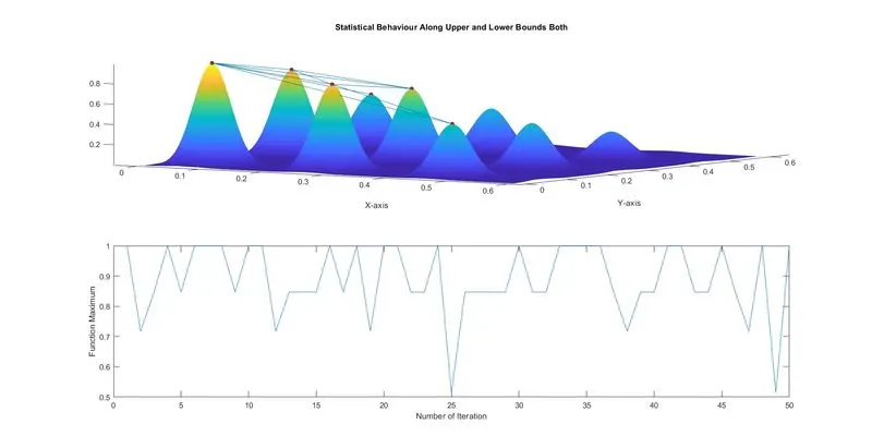
• The results of the above case will be different for each time when the program is runed. To get same value each time, we need to restrict the program within specific bounds namely upper bound and lower bound. The procedure for coding and plotting the procedure is same as Study 1. The only difference is in the ‘ga’ syntax. This time the algorithm is provided lower limits and upper limits as [0;0] and [1;1] respectively.
• After plotting the results of Study 2 or the bounded case, it is observed that the results are not same every time the program terminates. A solution to this problem is to increase the number of cases or iterations.
• Study 3, the number of iterations are increased to 300. So for this study, the syntax, “options = optimoptions(‘SolverName’,’Name’,‘Value’)” is used which returns with named parameter ‘Populations’ with the altering values ‘300’.
• The syntax ‘ga’ contains ‘option’ term and rest of the code is same as for Study 1 and 2 as process continues.

RESULTS:

Study1: Statistical Behaviour.

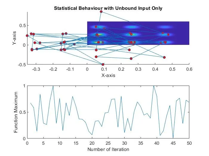
Large number of red dots shows values of co-ordinates of x, y varies each time iteration runs.

Study2:Statistical Behaviour with upper and lower bounds.

The number of red dots are less compared to previous plot. Result is providing upper and lower bounds to the function.

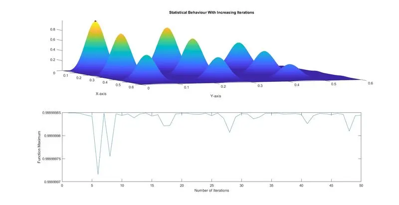
Study3:Statistical Behaviour with increasing iterations of Genetic Algorithm.

Number of iterations is increased to 300 to converge and find the global maxima of the function. Here we can see that there is only one red dot on the stalagmite function and that is the required global maxima point.Rotate the plot,the stalagmite function along with the global maxima value as x = 0.06683 and y = 0.06683 is calculated.

Refrence:

1. https://in.mathworks.com/help/gads/how-the-genetic-algorithm-works.html