Week 3 - Solving second order ODEs

objective : To Write a program for solving ODE representing the equation for the motion of a simple pendulum with damping using MATLAB.

a.Solving second order ODE along graph of Velocity v/s Displacement.

b.Creating the animation of the simple pendulum with video link.

Video Link for ODE simple pendulum : https://youtu.be/tWX9fxQgZbc

Description of ODE and Simple Pendulum:

An ordinary differential equation (ODE) is a differential equation containing one or more functions of one independent variable and the derivatives of those functions.

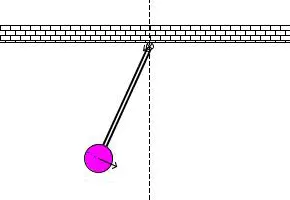
A simple pendulum can be described as a device where its point mass is attached to a light inextensible string and suspended from a fixed support. The vertical line passing through the fixed support is the mean position of a simple pendulum. The vertical distance between the point of suspension and the centre of mass of the suspended body (when it is in mean position) is called the length of the simple pendulum denoted by L. This form of the pendulum is based on the resonant system having a single resonant frequency.

Matlab Code Procedure:

Given -

Simulate the motion between 0-20 sec

for angular displacement = 0

angular velocity=3 rad/sec

at time t = 0

L = 1 metre

M = 1 kg

b = 0.05

g = 9.81 ms2

A] Code function of ode_func for main program:

function [dtheta_dt] = ode_func(t,theta,b,g,l,m)
theta1 = theta(1);
theta2 = theta(2);

dtheta1_dt = theta2
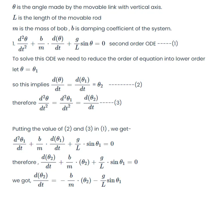
dtheta2_dt = (-(b/m)*theta2 - (g/l)*sin(theta1));
dtheta_dt = [dtheta1_dt;dtheta2_dt];

end

B]Simple Pendulum Full proram:

clear all
close all
clc

% Solving the Second order ODE and show the animation

% damping coefficient
b = 0.05;                     
% length of pendulum in metre
l = 1;                       
% mass of bob in kg
m = 1;   
% gravity in m/s^2
g = 9.81;                     

% Initial Condition
theta_0 = [0;3];

%Time points

t_span = linspace(0,20,500);

%Solve ODE 
[t,results] = ode45(@(t,theta) ode_func(t,theta,b,g,l,m),t_span,theta_0);

figure(1)
plot(t,results(:,1))
hold on
plot(t,results(:,2))
xlabel('Time')
ylabel('Velocity')
legend('Displacement','Angular velocity')
grid on
hold off

displacement = results(:,1);
velocity=results(:,2);

%fixed coordinates
x0=1;
y0=1;
ct=1;

for i = 1:length(displacement)
    
    %coordinates
    x1=1-l*sin(displacement(i));
    y1=1-l*cos(displacement(i));
    
    figure(2)
     %plot fixed link
     plot([0 2],[1 1],'linewidth',15,'color','b')
     hold on                              
     plot([1 x1],[1 y1],[x1 x1],[y1 y1],'-O','markersize',25,'markerfacecolor','r','linewidth',4)
     plot(x0,y0,'-O','markersize',3,'markerfacecolor','b')
     %axis setting
     axis([0 2 -0.5 2])

     % to change the frame of the movie
     M(ct)= getframe(gcf);                 
     ct=ct+1;
     hold off
end

movie(M)                                                                
videofile=VideoWriter('simple pendulum.avi','uncompressed AVI');
open(videofile)                                                         
writeVideo(videofile,M)                                                 
close(videofile)

Step wise Explanation of ODE simple pendulum program -

1.First, the given details are assigned as variables in the code.

2.Then time required for the simple pendulum is set by using linspace command then, theta value is given as a column matrix.

3.Then use ode_func function and call in main program.

4.Use plot command to plot graph corresponding to time and velocity,legend command is used for identify each values in the graph.

5.For having the accurate simulation of the simple pendulum corresponding to the second order ODE with damping their is need to use the looping statements, here FOR loop is used to create this.

6.Pendulum has fixed coordinates mentioned as x0,y0 and x1, y1 are some other coordinates.

7.MARKER command is used for making BOB of the pendulum, the axis is fixed using AXIS command.

8.The counter command is used to make the value changes in each for loop. And finally videoWriter command is used to create the video file.

Output:

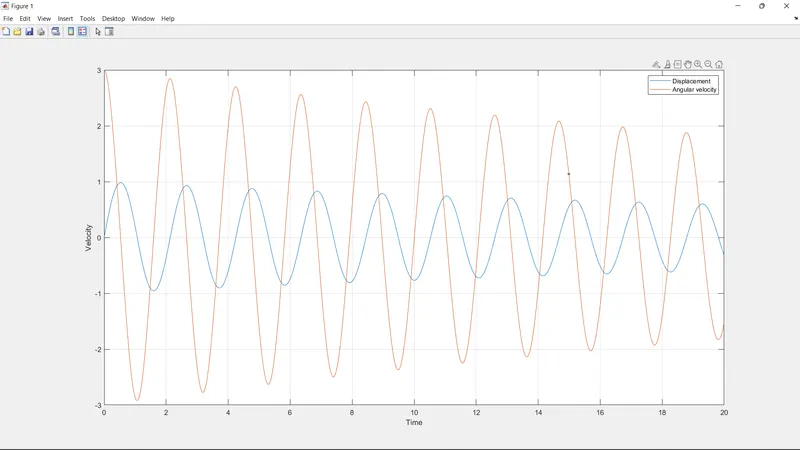
1.Graph of velocity v/s time which shows Displacement and Angular velocity.

2.Video Link for ODE simple pendulum : https://youtu.be/tWX9fxQgZbc

Error was occured:

Error occurd due to the slow running of program.

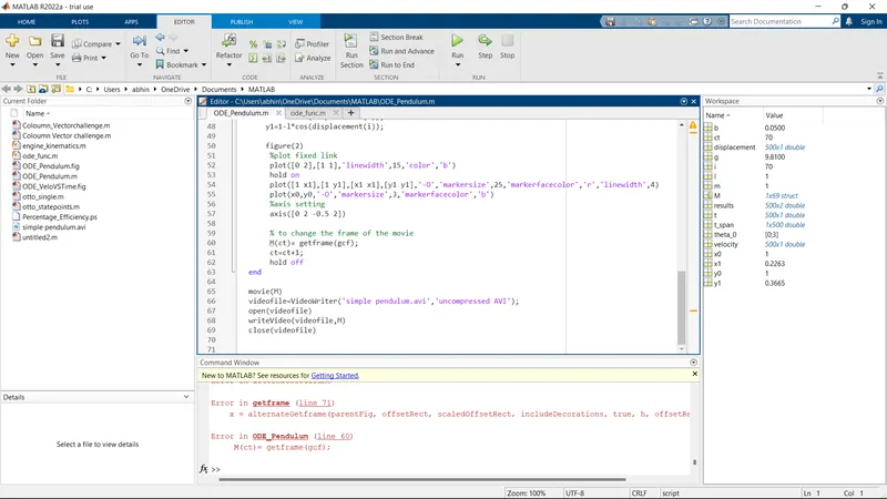
Error Removed by saving and running the full code again.