Week 4.1 - Genetic Algorithm

%genetic algorithum

clear all 
close all 
clc

%Defining our search space to be optimized.
%%one dimesional

x = linspace(0,0.6,150);
y = linspace(0,0.6,150);

%creating 2dimiensional grid
[x, y] = meshgrid(x,y);

% evaluating the stalagmite function

for i = 1:length(x);
    for j = 1:length(y);
        input_vector(1)= x(i,j);
        input_vector(2)= y(i,j);
        f(i,j) = stalagmite_func(input_vector);
    end

end

surfc(x,y,f)
shading interp

xlabel('x value')
ylabel('y value')
[x_output,fval] = ga(@stalagmite_func,2)

%stalegmite function defined
function v = stalagmite_func(input_vector)
x= input_vector (1) ;
y = input_vector (2);
f1_x = (sin(5.1*pi * x +0.5)).^6;
f1_y = (sin(5.1*pi * y +0.5)).^6;
f2_x = exp((-4*0.6931).*(x-0.0667)^2/(0.64));
f2_y = exp((-4*0.6931).*(y-0.0667)^2/(0.64));
v = -(f1_x.*f1_y.*f2_x.*f2_y);
end

%study 1 program
%Defining our search space to be optimized.
%%one dimesional
clc 
clear all
close all

x = linspace(0,0.6,150);
y = linspace(0,0.6,150);
num_cases=50;
%creating 2dimiensional grid
[x, y] = meshgrid(x,y);

% evaluating the stalagmite function

for i = 1:length(x);
    for j = 1:length(y);
        input_vector(1)= x(i,j);
        input_vector(2)= y(i,j);
        f(i,j) = stalagmite_func(input_vector);
    end

end
tic
for i=1:num_cases
    [inputs,fopt(i)]=ga(@stalagmite_func,2);
    xopt(i)=inputs(1);
    yout(i)=inputs(2);
end
study_time=toc
figure(1)
subplot(2,1,1)
hold on;
surfc(x,y,f)
shading interp
plot3(xopt,yout,fopt,'marker','o','markersize',5,'markerfacecolor','r')
subplot(2,1,2)
plot(fopt)

%study 2
% Defining our search space to be optimized.
%%one dimesional
clc 
clear all
close all

x = linspace(0,0.6,150);
y = linspace(0,0.6,150);
num_cases=50;
%creating 2dimiensional grid
[x, y] = meshgrid(x,y);

% evaluating the stalagmite function

for i = 1:length(x);
    for j = 1:length(y);
        input_vector(1)= x(i,j);
        input_vector(2)= y(i,j);
        f(i,j) = stalagmite_func(input_vector);
    end

end
tic
for i=1:num_cases
    [inputs,fopt(i)]=ga(@stalagmite_func,2,[],[],[],[],[0;0],[1;1]);
    xopt(i)=inputs(1);
    yout(i)=inputs(2);
end
study_time=toc
figure(2)
subplot(2,1,1)
hold on;
surfc(x,y,f)
shading interp
plot3(xopt,yout,fopt,'marker','o','markersize',5,'markerfacecolor','r')
subplot(2,1,2)
plot(fopt)
[x_output,fval] = ga(@stalagmite_func,2)

%study3
% Defining our search space to be optimized.
%%one dimesional
clc 
clear all
close all

x = linspace(0,0.6,150);
y = linspace(0,0.6,150);
num_cases=50;
%creating 2dimiensional grid
[x, y] = meshgrid(x,y);

% evaluating the stalagmite function

for i = 1:length(x);
    for j = 1:length(y);
        input_vector(1)= x(i,j);
        input_vector(2)= y(i,j);
        f(i,j) = stalagmite_func(input_vector);
    end

end
options=optimoptions('ga')
options=optimoptions(options,'populationSize',200)
tic
for i=1:num_cases
    [inputs,fopt(i)]=ga(@stalagmite_func,2,[],[],[],[],[0;0],[1;1],[],[],options);
    xopt(i)=inputs(1);
    yout(i)=inputs(2);
end
study_time=toc
figure(3)
subplot(2,1,1)
hold on;
surfc(x,y,f)
shading interp
plot3(xopt,yout,fopt,'marker','o','markersize',5,'markerfacecolor','r')
subplot(2,1,2)
plot(fopt)
[out,fval] = ga(@stalagmite_func,2)
 ginput(1)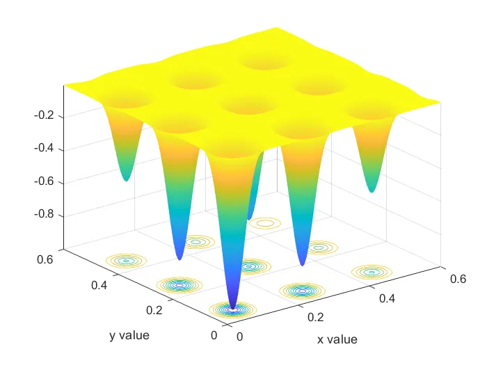

about gentic algorithms
ga is optimization technique this works same as the natural evalution process
in this process it select the best out come of the iteration the reject all other values or out comes
it starts the process do the itration select the best outcome of that iteration and reject remaining outcome the in second iteration select
among the first best out come
this technique is more ffective in optimation problem because as ga is know to find the best optimum solution

from the above knowledge we can say that more the number of iteration more accurete will be the result

now come to the challenge

Aim :-

1.find the globel maximum of the stalagmite function using ga function
2.understand the use of genentic algorithm
3.try to more get same output fro as many output

Governing eqn:
f(x,y)=f1_x*f1_y*f2_x*f2_y
f1_x=[sin(5.1*pi*x+0.5]^5
f1_y=[sin(5.1*pi*y+0.5]^5

f2_x=exp[-4log(2)*(x-0.0667)^2/0.64]
f2_y=exp[-4log(2)*(y-0.0667)^2/0.64]

Body of content:-
first stalagmite function is defined which is directly formula based function
the stalege mithe function has to done elementwise operation

now comes to the main program

x and y is divede to evaly spaced vector using linspace command then the vectory mesh graded
using for loop stalagmite function is calculated
using surf command the output is ploted
then using ga function otimum function is evaluated

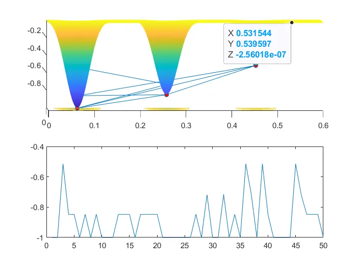
study-1
this same as above program but using this the output varies lot for every iteartion which can be seen in plot also
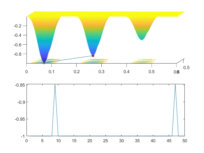
study 2
this process the upper and lower bound is defined due to this the simulation does take more time but the out variation is less as comparedto study 1

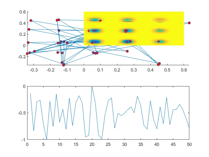
study 3
here population of the iteration increased as the iteration number increase the output is more acurate but it takes more time compred to above to simulation