Week 4.1 - Genetic Algorithm
AIM :
⁕ To understand the concept of genetic algarithm and write a code in MATLAB to optimise the stalagmite function and find the global maxima of the function.
THEORY
INTRODUCTION TO OPTIMIZATION :
Optimization is the process of making something better. In any process we have a set inputs and set of outputs as shown in the fig
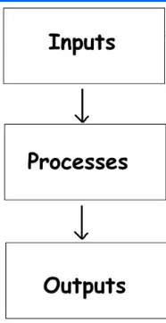
Optimization refers to finding the values of inputs in such a way that we get the "bear output values the definition of "pest varies from problem to problem, but in mathematical terms, it meters to maximizing or minimizing one or more objective function by varying the input parametern.
The set of all possible solutions or valdes which the inputs can take make up the search space in this search space lies o point or a setof points which gives the optimal solution. The aim of optimization is to find that paint or not of points in the search space.
In complex machine learning models, the performance usually depends on multiple input parameters. In order to get the optimal model, the parameters must be properly tuned. However, when there are multiple parameter variables, each ranging across a wide spectrum of values, there are too many possible configurations for each set of parameters to be tested. In these cases, optimization methods should be used to attain the optimal input parameters without spending vast amounts of time finding them.
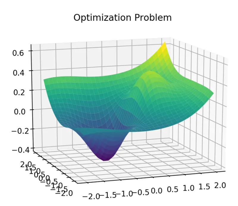
In the diagram above, it shows the distribution of the model based on only two parameters. As evident in the example shown, it is not always an easy task to find the maximum or minimum of the curve. This is why optimization methods and algorithms are crucial in the field of machine learning.
BASIC TERMINOLOGY
Before beginning a discussion on Genetic Algorithms, it is essential to be familiar with some basic terminology which will be used throughout this tutorial.
-
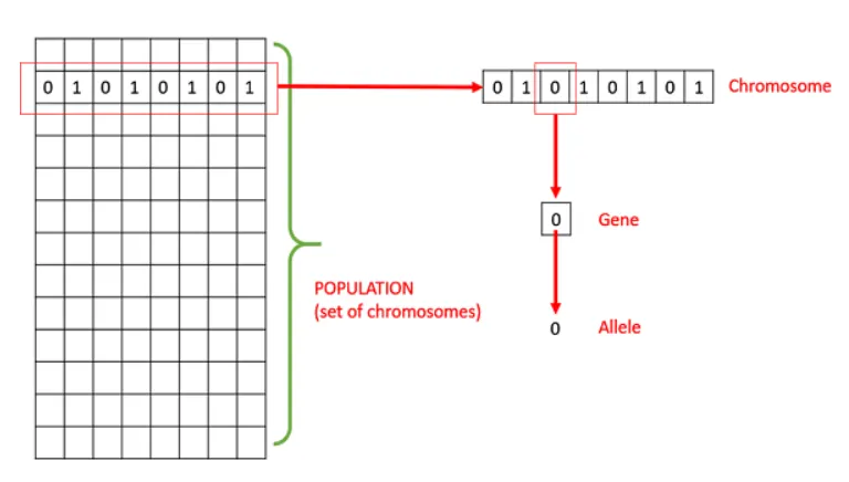
Population − It is a subset of all the possible (encoded) solutions to the given problem. The population for a GA is analogous to the population for human beings except that instead of human beings, we have Candidate Solutions representing human beings.
-
Chromosomes − A chromosome is one such solution to the given problem.
-
Gene − A gene is one element position of a chromosome.
-
Allele − It is the value a gene takes for a particular chromosome.
-
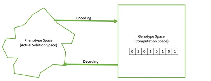
Genotype − Genotype is the population in the computation space. In the computation space, the solutions are represented in a way which can be easily understood and manipulated using a computing system.
-
Phenotype − Phenotype is the population in the actual real world solution space in which solutions are represented in a way they are represented in real world situations.
-
Decoding and Encoding − For simple problems, the phenotype and genotype spaces are the same. However, in most of the cases, the phenotype and genotype spaces are different. Decoding is a process of transforming a solution from the genotype to the phenotype space, while encoding is a process of transforming from the phenotype to genotype space. Decoding should be fast as it is carried out repeatedly in a GA during the fitness value calculation.
For example, consider the 0/1 Knapsack Problem. The Phenotype space consists of solutions which just contain the item numbers of the items to be picked.
However, in the genotype space it can be represented as a binary string of length n (where n is the number of items). A 0 at position x represents that xth item is picked while a 1 represents the reverse. This is a case where genotype and phenotype spaces are different.
-
Fitness Function − A fitness function simply defined is a function which takes the solution as input and produces the suitability of the solution as the output. In some cases, the fitness function and the objective function may be the same, while in others it might be different based on the problem.
-
Genetic Operators − These alter the genetic composition of the offspring. These include crossover, mutation, selection, etc.
Genetic Algorithms The most commonly used optimization strategy are Genetic Algorithms. Genetic Algorithms are based off of Darwin’s theory of natural selection. It is relatively easy to implement and there is a lot of flexibility for the setup of the algorithm so that it can be applied to a wide range of problems. FITNESS FUNCTION To start off, there must be a fitness function that measures how well a set of input parameters perform. Solutions with a higher fitness derived from a fitness function will be better than ones with a lower fitness.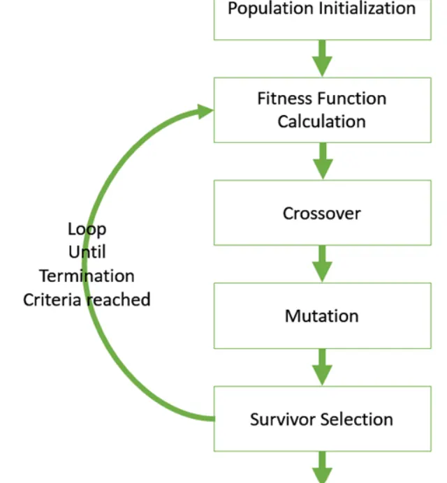


GENERATE A POPULATION
To run a genetic algorithm, first start off with a population of individuals where each individual is a solution. The solution is represented with a set of genes where each gene in the solution is a variable within the model. Each solution is randomly generated and evaluated against the fitness function to generate a fitness score. It is very important to choose an appropriate population size. If the population size is too low, then it is much harder to explore the entire state space of the problem. If the population is too large, then it will take a very long time to process each generation as system costs for calculating fitness and generating each population will take exponentially more time to process.
PARENT SELECTION
Next, the population goes through a process called parent selection where the best solutions (most fit individuals) will be selected to create the next generation of solutions. There are many ways to do this, such as Fitness-Proportion Selection (FPS), Rank-Based Selection, and Tournament Selection. These methods all have their pros and cons and should be picked based on the model.
CROSSOVER
Once the parents have been selected, the parents undergo a process called crossover. Crossover is when two parents crossover their genes in order to create a new solution (also known as a child). This promotes exploration in the state space of the problem and potentially generates new solutions that have never been tested before.
This is done differently based on the data types of the solutions. For solutions where the genes are represented in binary, there are methods such as 1-point crossover, n-point crossover, and uniform crossover.
For solutions where the genes are real-valued, there are methods such as single arithmetic crossover and whole arithmetic crossover.
Also, for permutation problems (such as the Traveling Salesman problem, etc) there are methods such as the Partially-Mapped Crossover (a.k.a. PMX), Edge crossover, Order 1 Crossover, and Cycle crossover.
MUTATION
After the crossover phase, the children generated goes through a mutation phase. Mutation is when each gene could potentially change according to a random probability. This allows for exploitation as the children solution will not change as drastically as during the crossover phase but will still be able to explore around the neighbourhood of its current solution.
For binary solutions, the mutation process is relatively simple where each bit is toggled according to some mutation probability.
For real-valued solutions, the different genes can be chosen according to some acceptable range for that variable or by adding some noise that centers around 0 and varies according to some Gaussian distribution.
Finally, for permutation problems, there are four main methods; insert mutation, swap mutation, inversion mutation, and scramble mutation.
SURVIVOR SELECTION
Once the children population is created, the next stage is survivor selection. This is the stage that decides which individuals get to move on to the next generation. There are multiple ways to do this as the new generation can be selected from both the pool of parents and the pool of children. There are two main methods to select the survivors of each generation, Age-Based Selection and Fitness-Based Selection (FBS). In FBS, there is Elitism, where the most fit of every population is selected, and Genitor, where the worst fit of every population gets eliminated.
ALGRITHM REPETITION
Once the new generation is selected, this whole process repeats until the algorithm converges based off of some convergence criteria. After the whole algorithm runs, the best solution from all of the generations is returned.
ADVANTAGES OF GAs
GAs have various advantages which have made them immensely popular. These include −
-
Does not require any derivative information (which may not be available for many real-world problems).
-
Is faster and more efficient as compared to the traditional methods.
-
Has very good parallel capabilities.
-
Optimizes both continuous and discrete functions and also multi-objective problems.
-
Provides a list of “good” solutions and not just a single solution.
-
Always gets an answer to the problem, which gets better over the time.
-
Useful when the search space is very large and there are a large number of parameters involved.
LIMITATIONS OF GAs
Like any technique, GAs also suffer from a few limitations. These include −
-
GAs are not suited for all problems, especially problems which are simple and for which derivative information is available.
-
Fitness value is calculated repeatedly which might be computationally expensive for some problems.
-
Being stochastic, there are no guarantees on the optimality or the quality of the solution.
-
If not implemented properly, the GA may not converge to the optimal solution.
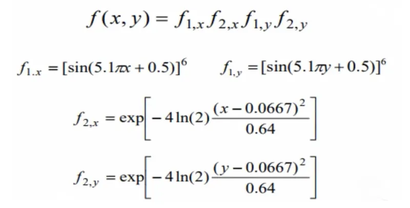
GOVERNING EQUATION FOR STALAGMITE FUNCTION :
MATLAB CODE FOR STALAGMITE FUNCTION
function [fmax] = stalagmite(input_vector)
x = input_vector(1);
y = input_vector(2);

f_1x = (sin((5.1*pi*x)+0.5))^6;
f_1y = (sin((5.1*pi*y)+ 0.5))^6;

f_2x = exp(-4*log(2)*((x - 0.0667)^2)/(0.64));
f_2y = exp(-4*log(2)*((y - 0.6667)^2)/(0.64));
fmax = -(f_1x*f_2x*f_1y*f_2y);
end

*****************************************************************************************
MAIN CODE FOR GENETIC ALGORITHM
close all
clear all
clc

% defining our search space
x = linspace(0,0.6,150);
y = linspace(0,0.6,150);

% creating a 3Dimensional mesh
[xx, yy] = meshgrid(x,y);

% evaluating the stalagmite function
for i = 1:length(xx)
    for j = 1:length(yy)
        input_vector(1)=xx(i,j);
        input_vector(2)=yy(i,j);
        f(i,j) = stalagmite(input_vector);
    end
end

surfc(xx,yy,-f)
shading interp

[inputs , fval] = ga(@stalagmite , 2);
xlabel('X axis')
ylabel('Y axis')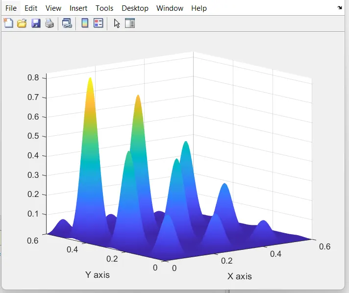
- Clear all, close all and clc represents it deletes all temporary memory, closes all plots, and clears the command window.
- We assume x and y values using the linspace command. The uses of linspace command are that if we set lower and upper limits and the number of values we need it takes random values.
- In the next step, the mesh grid command is used in order to form an array of row and column values and it is stored in xx and yy variables.
- Then, for loop command is used. It repeats the function for the length of xx and yy.
- Then in the next step, we call the stalagmite function as stalagmite(input_vector).
- In the next step, surfc command is used in order to get a plot as a surface.
- Then, shading interp command is used in order to remove the grid-like structure in the plot, and color filling is done.you can refer it in the following figure.
- In the next step, the ga command is used. In the ga command, we call the stalagmite function and we need to enter the number of variables. In our problem, we have two variables x and y so we enter it as 2.
- Then in the next step x label and y label is used in order to get a clear picture of our plot
clear all
close all
clc
%Defining our search space
x =linspace(0,.6,150);
y =linspace(0,.6,150);
num_case=50;
%creating a 2D mesh
[xx,yy]= meshgrid(x,y);

%evaluating the stalagmite function
for i=1:length(xx)
    for j =1:length(yy)
input_vector(1)=xx(i,j);
input_vector(2)=yy(i,j);
f(i,j)= stalagmite(input_vector);
    end
end

%case 1
tic
 for k = 1:num_case
     [inp,fval(k)] = ga(@stalagmite,2);
     x_1(k) = inp(1);
     y_1(k) = inp(2);
 end
 f = -f;
 fval = -fval;
study1_time=toc;

 figure (1)
 subplot(2,1,1)
 grid on
 surfc(xx,yy,f)
  hold on
 plot3(x_1,y_1,fval,'marker','o','markersize',5,'markerfacecolor','g')
 shading interp
 title('stalagmite plot')
 subplot(2,1,2)
 plot(fval,'color','r','LineWidth',1)
 xlabel ('X axis')
 ylabel('Y axis')
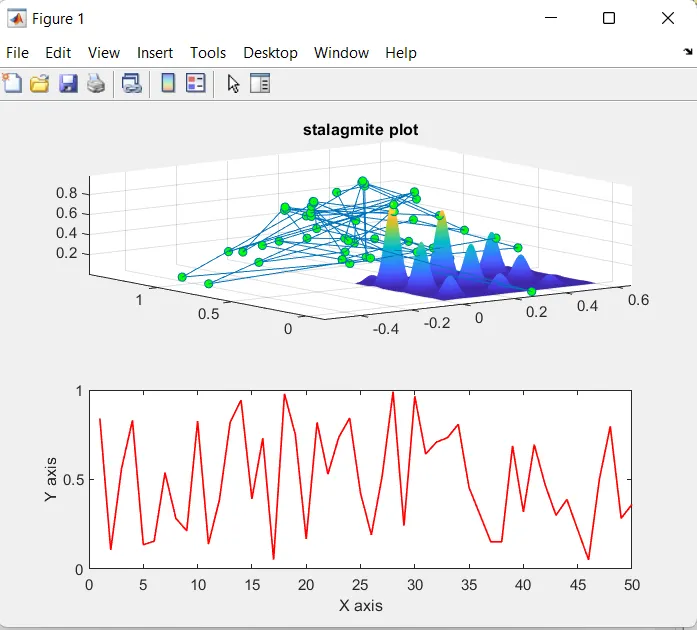
- In this study, we introduce the number of cases that ga needs to perform, and based on the mean value we need to calculate our global maximum value.
- We define it as num_cases=50 in this program. The 50 indicates that 50 times the ga need to repeat and it calculates the value.
- The tic command is used in order to find out the time taken for the program to complete.
- For loop command is used and the length of it set as the number of cases.
- Then ga command is used as before by calling the function and the number of variables in the program.
- The calculated x and y values are stored in xopt(i) and yopt(i).
- subplot command is used in order to get n number of plots in the same single figure plot.
- In the first plot, we plot the x,y, and f as a surface like structure by using the surf command.
- The negative sign is used in the function (f) while plotting since we invert initially and we need to revert it back to its original structure.
- Then we plot calculated maximum value as a dot-like structure by using the marker opting and marker size.
- In the next step title for the is mentioned using the title command.
- Then subplot command is used in order to plot in the same figure window.
- In this plot, we plot the values and the number of iterations, and the x label and y label is mentioned.
- In this study, we get a random value and we didn't get an exact global maximum value and the search space of ga is also not within our search space.
- Thus it indicates we need to have a better study method through which we get our exact global maximum value within our search space.
tic
 % study 2 - statistical behaviour with upper and lower bounds
 for k = 1:num_case
     [inp2,fval2(k)] = ga(@stalagmite,2,[],[],[],[],[0;0],[0.6;0.6]);
     x_2(k) = inp2(1);
     y_2(k) = inp2(2);
 end

 fval2= -fval2;
 study2_time=toc;

 figure (2)
 subplot(2,1,1)
 hold on
 surfc(xx,yy,f)
 shading interp
 plot3(x_2,y_2,fval2,'marker','o','markersize',5,'markerfacecolor','g')

 title('bounded inputs')
 subplot(2,1,2)
 plot(fval2,'color','r','LineWidth',1)
 xlabel ('X axis')
 ylabel('Y axis')
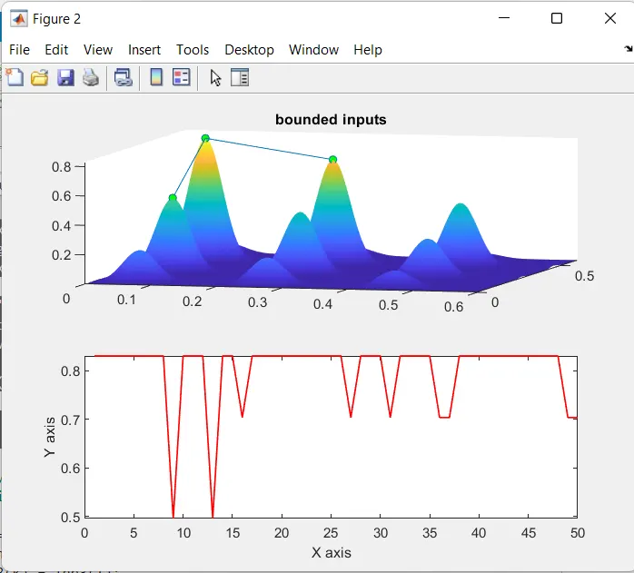
- From the previous study, we inferred that the search space of the ga is not within our search space so to overcome this error we use the bounded script method.
- As the name suggests, in this study we will enter the boundary and within that boundary, only the ga will perform.
- All the commands used in this study are also the same as used in the previous study except the ga syntax.
- In this study as mentioned above the limit criteria, Initially, we call the stalagmite function and the number of variables mentioned as done earlier, and we enter the lower and upper boundary limit values.
- In our program, the lower boundary limit is set as 0,0 and the upper boundary limit is set as 1,1.
- After this, we plot the same way as before and we get our plot.
- Based on the output we inferred that even though this study is better than our previous study but still we didn't an exact single global maximum value.
options = optimoptions('ga');
options = optimoptions(options,'PopulationSize',250);

% study 3 - statistical behaviour with upper and lower bounds
 %Defining our search space
tic
 for k = 1:num_case
     [inp3,fval3(k)] = ga(@stalagmite,2,[],[],[],[],[0;0],[0.6;0.6],[],[],options);
     x_3(k) = inp3(1);
     y_3(k) = inp3(2);
 end

 fval3= -fval3;
 study3_time=toc;

 figure (3)
 subplot(2,1,1)
  hold on
 surfc(xx,yy,f)

 shading interp
 plot3(x_3,y_3,fval3,'marker','o','markersize',5,'markerfacecolor','g')

 title('bounded inputs')
 subplot(2,1,2)
 plot(fval3,'color','r','LineWidth',1)
 xlabel ('X axis')
ylabel('Y axis') 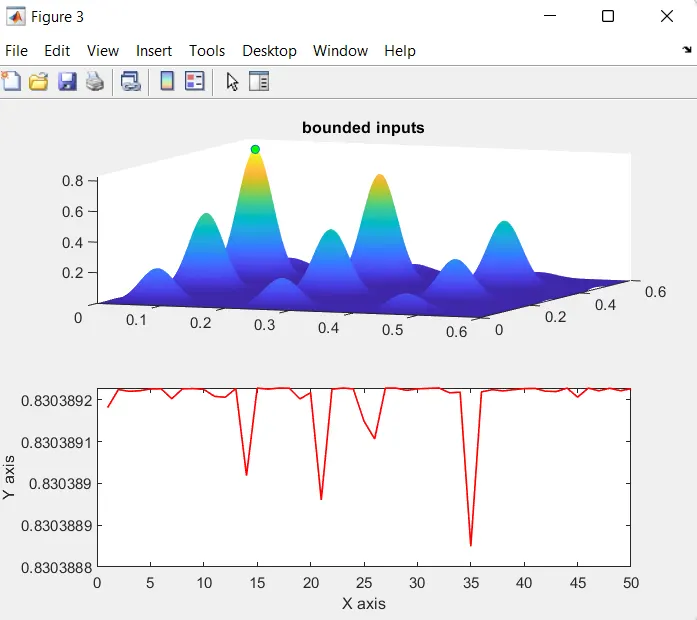
- All the commands used in this study are also the same as used in the previous study except the ga syntax.
- In the previous study, we set the lower and upper boundary limits but we didn't set the initial population size for the ga to perform.
- Thus in this optimization technique, we will try to set the initial population size that ga needs to perform within our boundary limits.
- Thus to set the initial population size we use the optimoptions command and in that we mention the options, population size.
- After this, we plot the same way as before and we get our plot.
- The population value is randomly increased up to which a single exact global maximum value is found out.
- By increasing like this we get a single exact point at the population size of 300.so we stop our program at this point.
Error:
The Errors were made which were simple syntax errors that are rectified right away with the help of the instructions in the command window.
Terms Used:
- Ga:
Ga function is used to find the minimum of the function using a genetic algorithm.
Syntax:
- For Random Inputs:
x = ga(fun,nvars) finds a local unconstrained minimum, x, to the objective function, fun. nvars is the dimension (number of design variables) of fun.
- For Bounded Inputs:
x = ga(fun,nvars,A,b,Aeq,beq,lb,ub) defines a set of lower and upper bounds on the design variables, x, so that a solution is found in the range lb ≤ x ≤ ub. (Set Aeq= [] and beq= [] if no linear equalities exist.)
- For Population size:
x = ga(fun,nvars,A,b,[],[],lb,ub,nonlcon,IntCon,options) requires that the variables listed in IntCon take integer values.
Where,
Fun - function,
Nvars – Number of Variables
A – Linear inequality constraints
B – Linear inequality constraints
Aeq - linear equality constraints
beq – linear equality constraints
lb – lower Bounds
ub – Upper Bounds
nonlcon – Non- Linear Constraints
IntCon – Integer Constraints
- Surfc:
surfc function contours the plot under the surface plot. surfc(X, Y, Z) creates a three-dimensional surface plot with a contour plot underneath. A surface plot is a three-dimensional surface that has solid edge colors and solid face colors. The function plots the values in matrix Z as heights above a grid in the x-y plane defined by X and Y. The color of the surface varies according to the heights specified by Z.
- Shading:
The shading function controls the color shading of surface and patch graphics objects.
Shading flat each mesh line segment and face has a constant color determined by the color value at the endpoint of the segment or the corner of the face that has the smallest index or indices.
shading faceted flat shading with superimposed black mesh lines. This is the default shading mode.
shading interp varies the color in each line segment and face by interpolating the colormap index or true color value across the line or face.
shading(axes_handle,...) applies the shading type to the objects in the axes specified by axes_handle, instead of the current axes. Use single quotes when using a function form. For example:
shading(gca,'interp')
- Plot3:
plot3(X, Y, Z) plots coordinates in 3-D space.
To plot a set of coordinates connected by line segments, specify X, Y, and Z as vectors of the same length.
To plot multiple sets of coordinates on the same set of axes, specify at least one of X, Y, or Z as a matrix and the others as vectors.
- Optimoptions:
options = optimoptions(SolverName) returns a set of default options for the SolverName solver.
options = optimoptions(oldoptions,Name,Value) returns a copy of oldoptions with the named parameters altered with the specified values.
- Tic- Toc:
tic works with the toc function to measure elapsed time. The 'tic' function records the current time, and the toc function uses the recorded value to calculate the elapsed time.
toc reads the elapsed time since the stopwatch timer started by the call to the tic function. MATLAB reads the internal time at the execution of the toc function and displays the elapsed time since the most recent call to the tic function without an output. The elapsed time is expressed in seconds.
RESULTS:
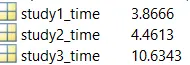
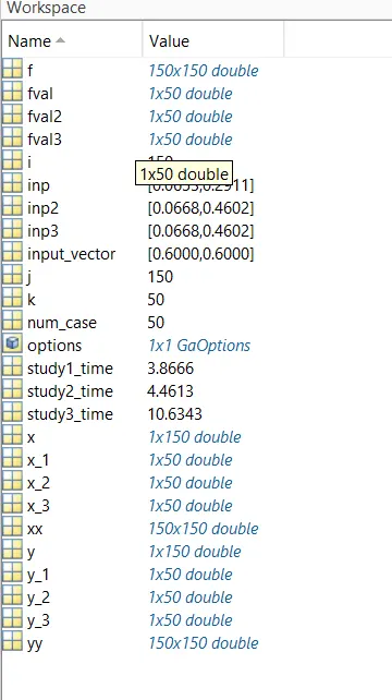
The time taken for the study, Global Maximum value and the coordinate values of x and y are found out for each study and the results are shown below
CONCLUSION:
- Understand how optimization technique is used with the ga command.
- Understand the function of ga and it uses.
- Understand how to improve our program step by step through different studies.
REFERENCE
https://towardsdatascience.com/optimizing-machine-learning-models-with-genetic-algorithms-2a38682a0610