Week 4.1 - Genetic Algorithm
AIM -
Write a code in MATLAB to optimise the stalagmite function and find the global maxima of the function.
OBJECTIVE -
Write a code using 'ga' function in MATLAB to optimise the stalagmite function and find the global maxima of the function. Testing for the most accurate plot using different syntax for 'ga' function, while discusing about gobla optimization , 'ga' syntax .
THEORY -
1.Genetic Algorithm -
Genetic Algorithm (GA) is a search-based optimization technique based on the principles of Genetics and Natural Selection. It is frequently used to find optimal or near-optimal solutions to difficult problems which otherwise would take a lifetime to solve. It is frequently used to solve optimization problems, in research, and in machine learning.
Nature has always been a great source of inspiration to all mankind. Genetic Algorithms (GAs) are search based algorithms based on the concepts of natural selection and genetics. GAs are a subset of a much larger branch of computation known as Evolutionary Computation.
GAs were developed by John Holland and his students and colleagues at the University of Michigan, most notably David E. Goldberg and has since been tried on various optimization problems with a high degree of success.
In GAs, we have a pool or a population of possible solutions to the given problem. These solutions then undergo recombination and mutation (like in natural genetics), producing new children, and the process is repeated over various generations. Each individual (or candidate solution) is assigned a fitness value (based on its objective function value) and the fitter individuals are given a higher chance to mate and yield more “fitter” individuals. This is in line with the Darwinian Theory of “Survival of the Fittest”.
In this way we keep “evolving” better individuals or solutions over generations, till we reach a stopping criterion.
Genetic Algorithms are sufficiently randomized in nature, but they perform much better than random local search (in which we just try various random solutions, keeping track of the best so far), as they exploit historical information as well.
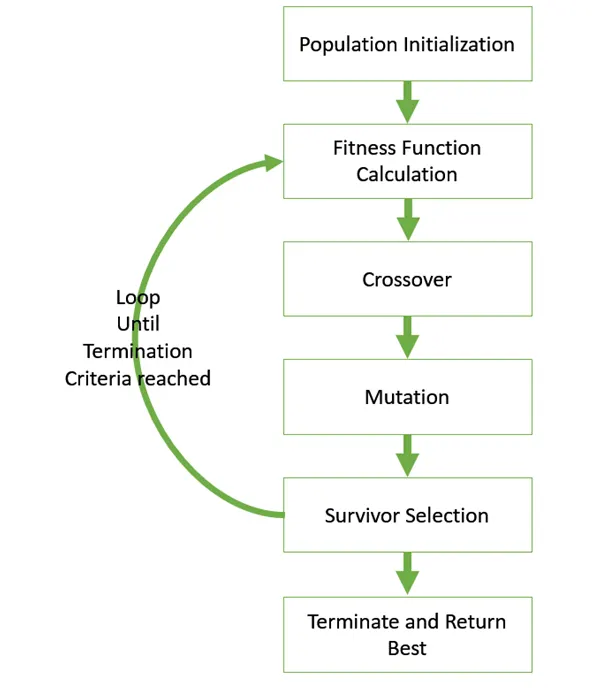
The basic structure of a GA −
We start with an initial population (which may be generated at random or seeded by other heuristics), select parents from this population for mating. Apply crossover and mutation operators on the parents to generate new off-springs. And finally these off-springs replace the existing individuals in the population and the process repeats. In this way genetic algorithms actually try to mimic the human evolution to some extent.
The following steps arefor a basic GA
2.Stalagmite Function -
Stalactite and stalagmite, elongated forms of various minerals deposited from solution by slowly dripping water. A stalactite hangs like an icicle from the ceiling or sides of a cavern. A stalagmite appears like an inverted stalactite, rising from the floor of a cavern.
A stalagmite function generally refers to the function with which we are generating values over a stalagmite kind of surface for finding out the local and global maxima and minima of that particular given function.

Formula for stalagmite function -
`f(x,y) = underset(1,x)(f).underset(2,x)(f).underset(1,y)(f).underset(2,y)(f)`
`underset(1,x)(f)= [sin(5.1pix+0.5)]^6`
`underset(1,y)(f)= [sin(5.1piy+0.5)]^6`
`underset(2,x)(f)= exp[-4ln(2)(x-0.0667)^2/0.64]`
`underset(2,y)(f)= exp[-4ln(2)(y-0.0667)^2/0.64]`
3. 'ga' function syntax -
x = ga(fun,nvars)- finds a local unconstrained minimum,
x, to the objective function,fun.nvarsis the dimension (number of design variables) offun.
x = ga(fun,nvars,A,b)- finds a local minimum
xtofun, subject to the linear inequalitiesA*x≤b.gaevaluates the matrix productA*xas ifxis transposed (A*x').
x = ga(fun,nvars,A,b,Aeq,beq)- finds a local minimum
xtofun, subject to the linear equalitiesAeq*x=beqandA*x≤b. (SetA=[]andb=[]if no linear inequalities exist.)gaevaluates the matrix productAeq*xas ifxis transposed (Aeq*x').
x = ga(fun,nvars,A,b,Aeq,beq,lb,ub)- defines a set of lower and upper bounds on the design variables,
x, so that a solution is found in the rangelb≤x≤ub. (SetAeq=[]andbeq=[]if no linear equalities exist.)
x = ga(fun,nvars,A,b,Aeq,beq,lb,ub,nonlcon)- subjects the minimization to the constraints defined in
nonlcon. The functionnonlconacceptsxand returns vectorsCandCeq, representing the nonlinear inequalities and equalities respectively.gaminimizes thefunsuch thatC(x)≤0andCeq(x) = 0. (Setlb=[]andub=[]if no bounds exist.)
x = ga(fun,nvars,A,b,Aeq,beq,lb,ub,nonlcon,options)- minimizes with the default optimization parameters replaced by values in
options. (Setnonlcon=[]if no nonlinear constraints exist.) Createoptionsusingoptimoptions.
x = ga(fun,nvars,A,b,Aeq,beq,lb,ub,nonlcon,intcon)- or
x= ga(fun,nvars,A,b,Aeq,beq,lb,ub,nonlcon,intcon,options)intcontake integer values.
x = ga(problem)- finds the minimum for
problem, a structure described inproblem.
[x,fval] = ga(___)- for any previous input arguments, also returns
fval, the value of the fitness function atx.
[x,fval,exitflag,output] = ga(___)- also returns
exitflag, an integer identifying the reason the algorithm terminated, andoutput, a structure that contains output from each generation and other information about the performance of the algorithm.
[x,fval,exitflag,output,population,scores] = ga(___)- also returns a matrix
population, whose rows are the final population, and a vectorscores, the scores of the final population.
MATLAB CODES -
1. Stalagmite Function code -
function [S] = stalagmite_max(input_vector)

x = input_vector(1)
y = input_vector(2)

f1_x = [sin(5.1*pi*x +0.5)].^6;
f1_y = [sin(5.1*pi*y +0.5)].^6;

f2_x = exp((-4*0.6931)*((x-0.0667).^2/0.64));
f2_y = exp((-4*0.6931)*((y-0.0667).^2/0.64));

S = -(f1_x * f1_y * f2_x * f2_y);
end
Explanation -
- In this function code we calculate the values of x,y to get the stalagmite value by which we cam get the global maxima.
2. Final code to optimise the stalagmite function and find the global maxima of the function -
clear all
close all
clc

%defining research space
x= linspace(0,0.6,150);
y= linspace(0,0.6,150);

num_cases = 100;

%creating a 2D mesh
[xx yy] =meshgrid(x,y);

%evaluating stalagmite function
for i=1:length(xx)
    for j=1:length(yy)
        input_vector(1) = xx(i,j);
        input_vector(2) = yy(i,j);
        f(i,j) = stalagmite_max(input_vector);
    end
end

%study1 stastical behavior
tic
for i=1:num_cases
    [inputs,fopt(i)] = ga(@stalagmite_max,2);
    xopt(i) = inputs(1);
    yopt(i) = inputs(2);
end

study1_time = toc

fopt=-fopt

figure(1)
subplot(2,1,1);
hold on
surfc(xx,yy,-f)
shading interp
plot3(xopt,yopt,fopt,'Marker','o','markersize',5,'MarkerFaceColor','r')
title('Unbounded Inputs')
subplot(2,1,2)
plot(fopt)
xlabel('Iteration')
ylabel('Function Maximum')

%study2 stastical behavior with upper and lower bounds
tic
for i=1:num_cases
    [inputs,fopt(i)] = ga(@stalagmite_max,2,[],[],[],[],[0;0],[1;1]);
    xopt(i) = inputs(1);
    yopt(i) = inputs(2);
end

study2_time = toc

fopt=-fopt

figure(2)
subplot(2,1,1);
hold on
surfc(xx,yy,-f)
shading interp
plot3(xopt,yopt,fopt,'Marker','o','markersize',5,'MarkerFaceColor','r')
title('Bounded Inputs')
subplot(2,1,2)
plot(fopt)
xlabel('Iteration')
ylabel('Function Maximum')

%study3 stastical behavior with more GA iterations
options = optimoptions('ga');
options = optimoptions(options,'PopulationSize',500);

tic
for i=1:num_cases
    [inputs,fopt(i)] = ga(@stalagmite_max,2,[],[],[],[],[0;0],[1;1],[],[],options);
    xopt(i) = inputs(1);
    yopt(i) = inputs(2);
end

study3_time = toc

fopt=-fopt

figure(3)
subplot(2,1,1);
hold on
surfc(xx,yy,-f)
shading interp
plot3(xopt,yopt,fopt,'Marker','o','markersize',5,'MarkerFaceColor','r')
title('Increased Population')
subplot(2,1,2)
plot(fopt)
xlabel('Iteration')
ylabel('Function Maximum')
Explanation & Results -
-
First we initialise the values of x and y taking 150 values between the interval 0 and 0.6, We consider no of iterations 100.
-
Since we need to plot a 3D surface plot we take the 2d array of x and y using meshgrid command and store them in input_vector array ,so that it can be used as an argument to call the function stalagmite we create another function file for the stalagmite function. here we take the ouput as -f since ga only minimises a given function.so if -f is considered it automatically gives us the maxima.
- Now for Study case 1 -
We take num_cases value and we use the genetic algorithm function to caluclate the maxima of the function. we store the outputs into results which contain maximas and fopt which contain the value at which the maxima is obtained.
Here the ga is initiated with random population.
Then store the results into xopt, yopt.now we need to plot the surface of x,y,-f to get the 3D plot.
We use the plot3 command to make a plot of xopt,yopt and -fopt to plot the optimum maximas.
Also let us plot the fopt function so that we can visualise the optimum values at each iteration.
To get the time taken to complete cycle we used the tic toc commands to record the time.
The executed study 1 output is displayed as -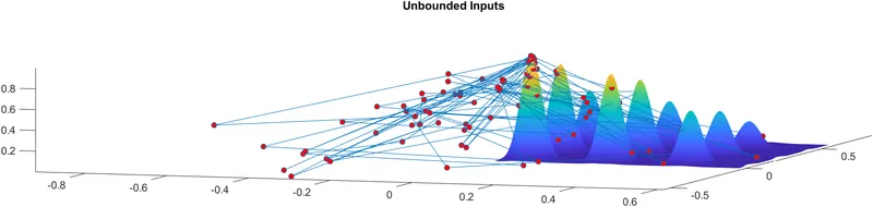
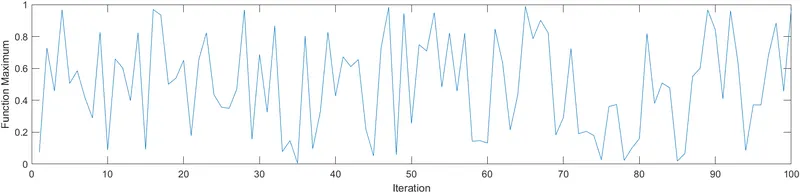
Here we can see the optimal values went outside the values of x and y resulting in falling away from stagalmite surface.
So we failed to reach the global maxima in this case.
the study 1 time = 160.3841s
- Now for Study case 2 -
let us specify the lower and upper bounds of x and y in this case,the ga is initiated with random population only.
Then we ploted the same way as study case 1.
The executed study 2 output is displayed as -
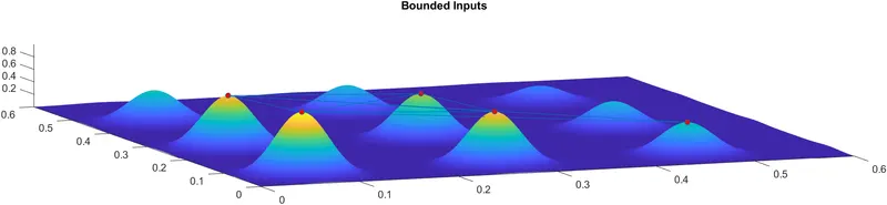
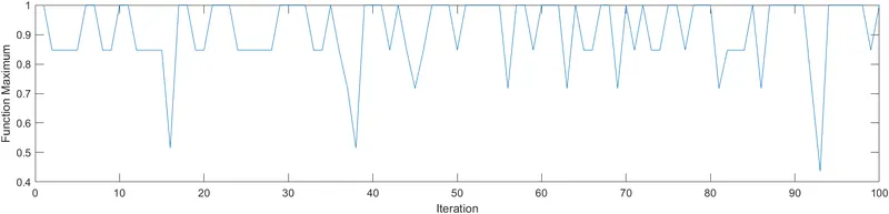
Though the optimum values are within the limits it could not give us the exact maxima values.
The study 2 time = 141.8880s
- Now for Study case 3 -
In this case let us increase our initial population which is default as 100 to 500.
Here in this case to set a initial population we need to use command called optimumoptions and get our value of 'populationsize' to 500.
Then we ploted the same way as previous plots.
The executed study 3 output is displayed as -
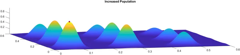
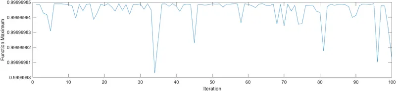
Though the time of execution is more in this case we are sucessfully to find out the correct global maxima for the stalagmite function.
So by increasing the initrial population size of the ga we can increase the accuracy of the algorithm.
The study 3 time = 1.2984e+03 s which is more than above two studies.