Project 1 - Parsing NASA thermodynamic data
AIM -
Aim of this project is to write a code in MATLAB to parse the NASA thermodynamic data file and then calculate Specific Heat(Cp), Enthalpy(H) and Entropy(S) for the local temperature range, Molecular Weight and Plot nature of the thermodynamic properties of given different species.
OBJECTIVE -
- Write a function that extracts the 14 co-efficients and calculates the enthalpy, entropy and specific heats for all the species in the data file.
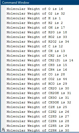
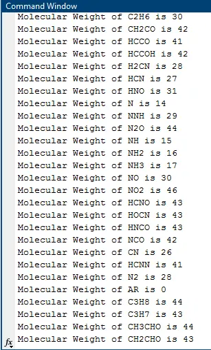
- Calculate the molecular weight of each gas species and display it in the command window.
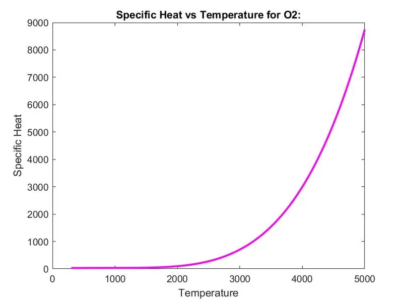
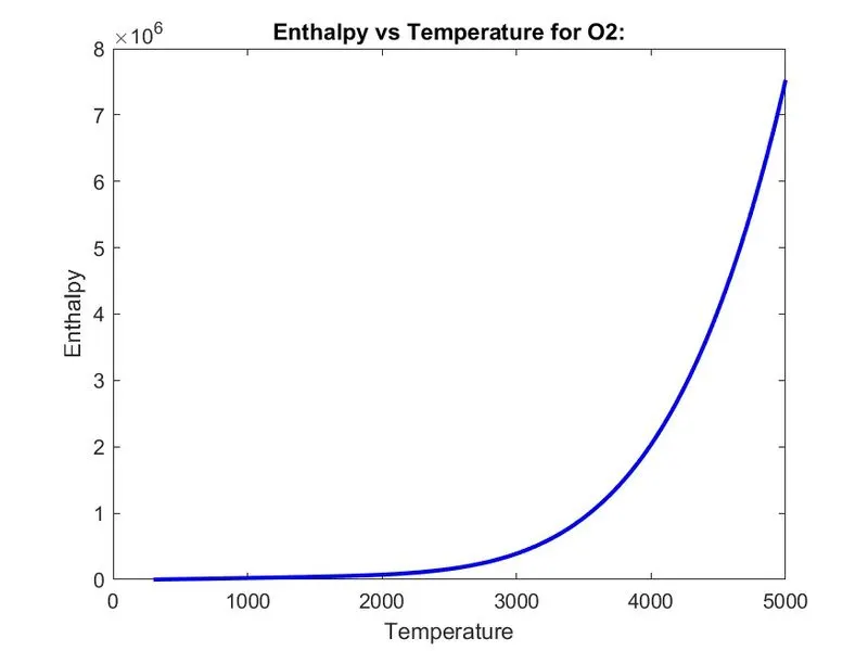
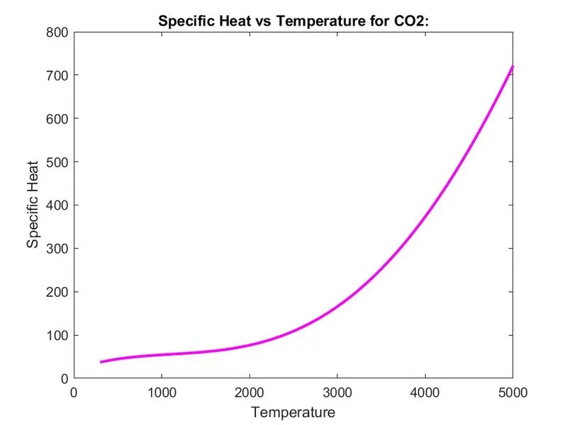
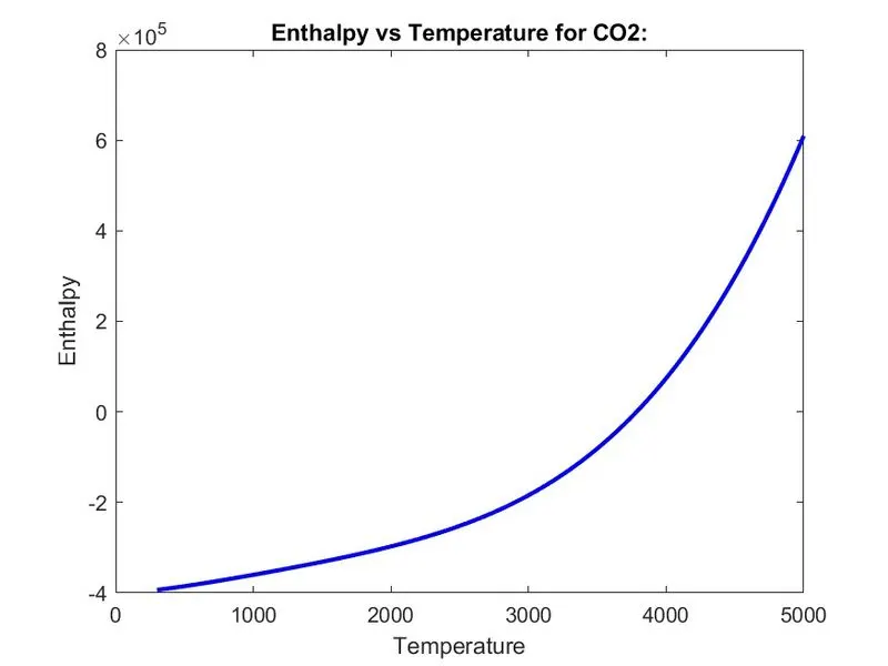
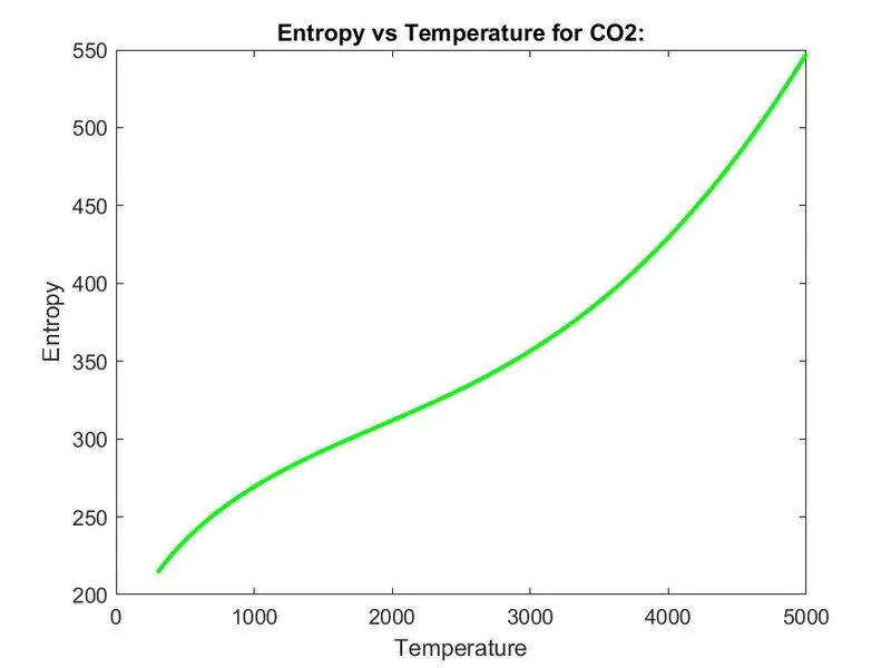
- Plot the Specific Heat(Cp), Enthalpy(H) and Entropy(S) for the local temperature range specific for each gas species.
THEORY -
1. Thermodynamics -
Thermodynamics, Science of the relationship between heat, work, temperature and energy. In broad terms, thermodynamics deals with the transfer of energy from one place to another and from one form to another. The key concept is that heat is a form of energy corresponding to a definite amount of mechanical work.
- Specific heat(Cp), the quantity of heat required to raise the temperature of one gram of a substance by one Celsius degree. The units of specific heat are usually calories or joules per gram per Celsius degree. For example, the specific heat of water is 1 calorie (or 4.186 joules) per gram per Celsius degree.
- Enthalpy(H) is the measurement of energy in a thermodynamic system. The quantity of enthalpy equals to the total content of heat of a system, equivalent to the system's internal energy plus the product of volume and pressure.
- Entropy(S), the measure of a system's thermal energy per unit temperature that is unavailable for doing useful work. Because work is obtained from ordered molecular motion, the amount of entropy is also a measure of the molecular disorder, or randomness, of a system.
Formulas used in this project -
- Specific Heat (Cp)
`Cp=R(a1+a2T+a3T^2+a4T^3+a5T^4)`
- Enthalpy(H)
`H =RT(a1+a2T/2+a3T^2/3+a4T^3/4+a5T^4/5+a6/T)`
- Entropy(S)
`S=R(a1lnT+a2T+a3T^2/2+a4T^3/3+a5T^4/4+a7)`
2. File Parsing -
Parsing a file means reading in a data stream of some sort and building an in memory model of the semantic content of that data. In otherwords, file parsing refers to how information can be read from a particular text file or any type of file and how that information can be used to in a computer program.
Text parsing is a common programming task that splits the given sequence of characters or values(text) into smaller parts based on some rules. It has been used in a wide variety of applications ranging from simple file parsing to large scale natural language processing. For example, NASA came up with polynomials such as Cp,H and S. They have also documented the co-efficients that are required to evaluate these polynomials for 1000+ species.
MATLAB CODE -
1.Function to calculate the Specific Heat
function Cp = specific_heat(a1,a2,a3,a4,a5,a6,a7,b1,b2,b3,b4,b5,b6,b7,R,temp,global_min_temp,global_max_temp,global_mid_temp)

if temp<=global_mid_temp
       Cp = R*(a1 + a2.*temp + a3.*(temp.^2) + a4.*(temp.^3) + a5.*(temp.^4));

else
       Cp = R*(b1 + b2.*temp + b3.*(temp.^2) + b4.*(temp.^3) + b5.*(temp.^4));
end
end
Explanation -
- This function uses the high-temperature coefficients, low-temperature coefficients, universal gas constant, and global minimum, global mid and global maximum temperature values as the input parameters.
- Then we use the ‘if else’ conditional statement to check if the temp values are less than or equal to the global middle temperature values and select the appropriate equations with high and low-temperature coefficients is used to calculate the specific heat value denoted by Cp and return that value.
2.Function to calculate the Enthalpy
function H = enthalpy(a1,a2,a3,a4,a5,a6,a7,b1,b2,b3,b4,b5,b6,b7,R,temp,global_min_temp,global_max_temp,global_mid_temp)

if temp <=global_mid_temp
        H = R.*temp.*(a1 + a2.*(temp./2) + a3.*((temp.^2)./3) + a4.*((temp.^3)./4) + a5.*((temp.^4)./5) + a6./temp);
else
        H = R.*temp.*(b1 + b2.*(temp./2) + b3.*((temp.^2)./3) + b4.*((temp.^3)./4) + b5.*((temp.^4)./5) + b6./temp);

end
end
Explanation -
- This function uses the high-temperature coefficients, low-temperature coefficients, universal gas constant, and global minimum, global mid and global maximum temperature values as the input parameters.
- Then using the ‘if else’ conditional statement the temp values is compared with the global middle temperature values and the appropriate equation with the proper maximum or minimum temperature coefficients is selected and the enthalpy is calculated and its value represented by H is returned.
3.Function to calculate the Entropy
function S = entropy(a1,a2,a3,a4,a5,a6,a7,b1,b2,b3,b4,b5,b6,b7,R,temp,global_min_temp,global_max_temp,global_mid_temp)


if temp<=global_mid_temp
        S = R*(a1.*log(temp) + a2.*temp + a3.*(temp.^2)./2 + a4.*(temp.^3)./3 + a5.*(temp.^4)./4 + a7);

else
        S = R*(b1.*log(temp) + b2.*temp + b3.*(temp.^2)./2 + b4.*(temp.^3)./3 + b5.*(temp.^4)./4 + b7);
end
end
Explanation -
- This function uses the high-temperature coefficients, low-temperature coefficients, universal gas constant, and global minimum, global mid and global maximum temperature values as the input parameters.
- Then using the ‘if else' conditional statement the temp values are compared with the global middle temperature values and the appropriate equation with the proper maximum or minimum temperature coefficients is selected and the entropy is calculated and its value represented by S is returned.
4.Function to calculate the molecular weight
function [W] = molecular_weight(element_name)

Str = {'H' 'C' 'N' 'O' 'AR'};

%atomic weight of each elements
gas_wt = [1 12 14 16 40];
W = 0;

for i = 1:length(element_name)
    for j = 1:length(Str)
        if strcmp(element_name(i), Str(j))
            W= W + gas_wt(j);
            %storing the position of matched element
            position = j;
        end
    end
    n = str2double(element_name(i));
    if n > 1
        W = W + gas_wt(position)*(n-1);
    end
end
end
Explanation -
- This function for molecular weight calculations requires element name as input argument and it is saved in the variable 'element_name' and the output argument is molecular weight.
- A string array is created which contains the name of the gases.
- A variable gas_wt is created which contains the atomic weight of respective atoms in the string array.
- Then used ‘strcmp’ command to compare the name of the element with the string array.
- If there is a repetition of an element, ‘str2double’ is used to find that and (n-1) is multiplied to gas_wt of the element to calculate molecular weight.
5.Function to write the molecular weight data of all elements to a file
function mol_wt_file(element_name,weight)

file_name = element_name;
mol_file = fopen('mol_wt.dat','a+');
fprintf(mol_file, 'Molecular weight of %s is %f n', file_name,weight);
fclose(mol_file);

end
Explanation -
- Firstly a new file is created with name 'mol_wt.dat' and it is opened in append mode denoted by 'a+' so that we can write the molecular weight of all elements in a single file.
- Using the ‘fprintf’ command the name of the element along with their molecular weight is written to the file.
6.Function to plot and save the graphs
function plot_fun(Cp,H,S,temp,element_name)
cd(pwd);
file_name=element_name;
%to create a new folder in the current directory
mkdir(file_name);

%Plotting Temperature vs specific heat
figure(1)
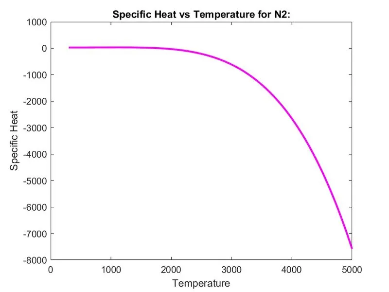
plot(temp,Cp,'lineWidth',2,'color','m');
title(sprintf('Specific Heat vs Temperature for %s:',element_name));
xlabel('Temperature');
ylabel('Specific Heat');

% Plotting Temperature vs Enthalpy
figure(2)
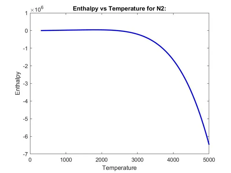
plot(temp,H,'linewidth',2,'color','b');
title(sprintf('Enthalpy vs Temperature for %s:',element_name));
xlabel('Temperature');
ylabel('Enthalpy');

% Plotting temperature vs Entropy
figure(3)
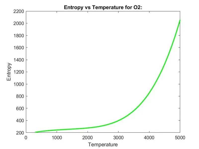
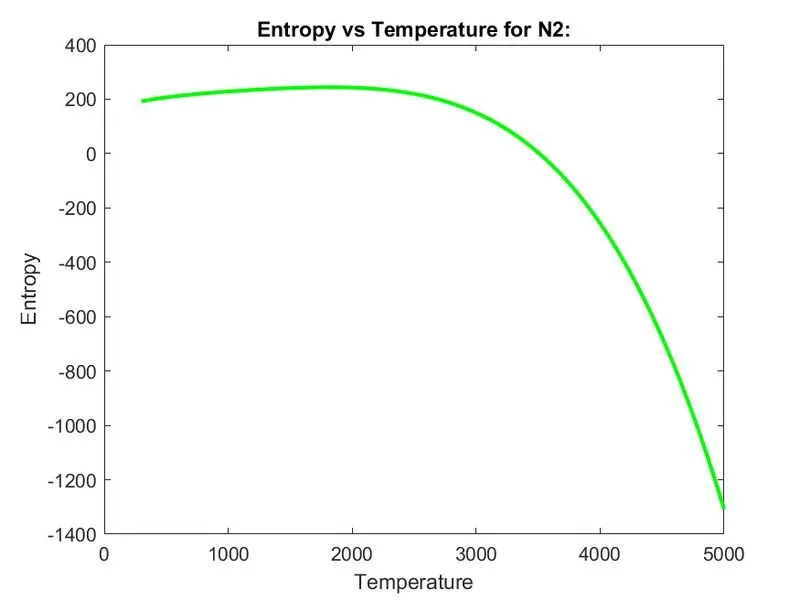
plot(temp,S,'linewidth',2,'color','g');
title(sprintf('Entropy vs Temperature for %s:',element_name));
xlabel('Temperature');
ylabel('Entropy');
cd(file_name);

path = 'F:\Course\HEVD&A\MATLAB for ME\Project\Project-1';

    plot_1 = fullfile(path,element_name,'Specific_Heat_vs_Temperature_Plot.jpg');
    plot_2 = fullfile(path,element_name,'Enthalpy_vs_Temperature_Plot.jpg');
    plot_3 = fullfile(path,element_name,'Entropy_vs_Temperature_Plot.jpg');

    saveas(figure(1),plot_1)
    saveas(figure(2),plot_2)
    saveas(figure(3),plot_3)

cd ..

end
Explanation -
- Using the ‘mkdir’ command a new folder is created in the current folder ‘pwd’ with the same name as the element name.
- The figure(1) represents the plots for temperature vs specific heat values.
- The figure(2) represents the plots for temperature vs enthalpy values.
- The figure(3) represents the plots for temperature vs entropy values.
- Giving the path to where the plots will be saved
- Using the ‘saveas’ command the three figures are saved in the new folder which is created by the element name.
- Using the ‘cd’ command the folder is changed back to the original folder.
- The function runs for 53 times through the ‘for’ loop and it creates separate folders for each species and saves all the plots in the folders.
7.Final CODE to calculate NASA Thermodynamic data
clear all
close all
clc

%Universal Gas Constant in J/(mol*K)
R= 8.314;

%Reading the data file
TH = fopen('THERMO.dat','r');

%Reading the first line of the file% creates a new folder in the current directory
L1 = fgetl(TH);

%Getting the global minimum, maximum and middle temperatures
L2 = fgetl(TH);
t = strsplit(L2);
global_min_temp = str2double(t{2});
global_mid_temp = str2double(t{3});
global_max_temp = str2double(t{4});

%Defining the temperature range
temp = linspace(global_min_temp,global_max_temp,500);

%Ignoring the comments in the file
for i=1:3
fgetl(TH);
end

for i=1:53
    %Reading the first line which includes the information for species
    l=fgetl(TH);

    %Reading the name of the species
    element_name=strtok(l);

    %Reading the three lines which contains 7 high temp coefficients & 7 low temp coefficients
    l1=fgetl(TH);
    l2=fgetl(TH);
    l3=fgetl(TH);

    %Finding the position of E so that we can extract the coefficients
    a=strfind(l1,'E');
    b=strfind(l2,'E');
    c=strfind(l3,'E');

    %Extracting high temp coefficient
    a1=str2double(l1(1:a(1)+3));
    a2=str2double(l1(a(1)+3:a(2)+3));
    a3=str2double(l1(a(2)+4:a(3)+3));
    a4=str2double(l1(a(3)+4:a(4)+3));
    a5=str2double(l1(a(4)+4:a(5)+3));
    a6=str2double(l2(1:b(1)+3));
    a7=str2double(l2(b(1)+4:b(2)+3));

    %Extracting low temp coefficient
    b1=str2double(l2(b(2)+4:b(3)+3));
    b2=str2double(l2(b(3)+4:b(4)+3));
    b3=str2double(l2(b(4)+4:b(5)+3));
    b4=str2double(l3(1:c(1)+3));
    b5=str2double(l3(c(1)+4:c(2)+3));
    b6=str2double(l3(c(2)+4:c(3)+3));
    b7=str2double(l3(c(3)+4:c(4)+3));

    %Calculating specific heat (kJ/kg-K)
    Cp = specific_heat(a1,a2,a3,a4,a5,a6,a7,b1,b2,b3,b4,b5,b6,b7,R,temp,global_min_temp,global_max_temp,global_mid_temp);

    %Calculalting enthalpy (kJ)
    H = enthalpy(a1,a2,a3,a4,a5,a6,a7,b1,b2,b3,b4,b5,b6,b7,R,temp,global_min_temp,global_max_temp,global_mid_temp);

    %Calculating entropy (kJ/K)
    S = entropy(a1,a2,a3,a4,a5,a6,a7,b1,b2,b3,b4,b5,b6,b7,R,temp,global_min_temp,global_max_temp,global_mid_temp);

    %Calculating molecular weights
    mol_wt(i) = molecular_weight(element_name);
    disp(['Molecular Weight of ',element_name,' is ',num2str(mol_wt(i))])

    %Function to write molecular weight to a file
    weight = mol_wt(i);
    mol_wt_file(element_name,weight);

    %Plotting graphs for Cp vs Temp, H vs Temp and S vs Temp plots for all the gases
    plot_fun(Cp,H,S,temp,element_name);


end
fclose(TH)
Explanations -
- First the value of the universal gas constant R is given as 8.314 as an input.
- Then using the ‘fopen’ command and read mode specified by 'r' we read the file named 'THERMO.dat'.
- Using the ‘fgetl’ command read first line which represents the title if the file so it is ignored.
- The next line has the global maximum, global middle and global minimum temperature values which is read by using ‘fgetl’ command and split into the three values by using the ‘strsplit’ command and converted into numbers.
- Then the temperature array is defined using ‘linspace’ command as 500 values between the global minimum and global maximum values.
- The next three lines are comments in the file so they are ignored by using a ‘for’ loop to iterate for 3 values.
- Then a ‘for’ loop is created to loop through the 53 species data given in the file and calculate the required values.
- Inside the loop, the ‘fgetl’ command is used to read the next line of the file which represents the name of the species, name of the element is stored in a variable using ‘strtok’ command.
- Then the next 3 lines of the file is read which contains the high and low temperature data of the particular species.
- The read lines are in the form of a string so they are converted into numbers using the ‘str2double’ command and stored in specific variables so they can be used for further calculations.
- The low temperatures values are stored in variables a1,a2,a2,a4,a5,a6 and a7 and the high temperature values are stored invariables b1,b2,b3,b4,b5,b6 and b7.
- The next line calculates and returns the value of specific heat using the high and low-temperature values as inputs using newly created specific heat funtion.
- The next line calculates and returns the value of enthalpy using the high and low-temperature values as inputs using newly created enthalpy funtion.
- The next line calculates and returns the value of entropy using the high and low-temperature values as inputs using newly created entropy funtion.
- The next line is the reference to 'molecular_weight' function that calculates the molecular weights of the different elements and displays the values in the command window.
- The next line is the reference to 'mol_wt_file' function that writes the molecular weights of different elements to a file.
- Then using plot_fun function plotting the graphs for every gas.
- The nasa_thermo_code file is closed using the ‘fclose’ command.
Results -
1.The molecular weight of each species displayed it in the command window
2.1. Plots for O2
I. Specific Heat & Temperature Plot
II. Enthalpy & Temperature Plot
III. Entropy & Temperature Plot
2.2. Plots for N2
I. Specific Heat & Temperature Plot
II. Enthalpy & Temperature Plot
III. Entropy & Temperature Plot
2.3. Plots for CO2
I. Specific Heat & Temperature Plot
II. Enthalpy & Temperature Plot
III. Entropy & Temperature Plot
3. Screenshot of the windows where all element folders are saved

Conclusion -
- This file parsing project includes several modules like finding correct information, converting them to useful form, plotting the relations and saving them automatically at the correct location. All the tasks led to great learning of various functions related to file handling in MATLAB. This project was interesting and challenging to complete.
Reference -
- https://in.mathworks.com/help/matlab/ref/mkdir.html
- https://in.mathworks.com/matlabcentral/answers/317006-create-new-folders-by-mkdir
- https://in.mathworks.com/help/matlab/ref/saveas.html
- https://in.mathworks.com/matlabcentral/answers/17580-how-to-define-a-path-in-saveas-command
- https://in.mathworks.com/help/matlab/referencelist.html?type=function&category=printing-and-exportinghttps://in.mathworks.com/help/matlab/ref/fprintf.html
- https://in.mathworks.com/help/matlab/ref/sprintf.html