Week 4.1 - Genetic Algorithm

1. code in MATLAB to optimise the stalagmite function and find the global maxima of the function.

%Creating the search space to be optimized
%one dimensional

clear 
close all
clc
n=150;
x = linspace(0,0.6,150);
y = linspace(0,0.6,150);
tic

%creating two dimensional grid
[xx, yy] = meshgrid(x,y);

%evaluating the stalagmite function

for i = 1:length(xx)
    for j = 1:length(yy)
        input_vector(1)= xx(i,j);
        input_vector(2)= yy(i,j);
        f(i,j) = stalagmite(input_vector);
    end
end

figure(1)
surfc(xx, yy, -f)
shading interp
xlabel('x value');
ylabel('y value');
study_time=toc;

% first case (unbounded inputs)
tic
for i = 1:n
    [inputs,fopt(i)]=ga(@stalagmite,2);
    xopt(i)=inputs(1);
    yopt(i)=inputs(2);
end

figure(2)
subplot(2,1,1)
hold on
surfc (x,y,-f)
shading interp
plot3(xopt,yopt,-fopt,'marker','o','markersize',5,'markerfacecolor','r')
title('unbounded inputs')
subplot(2,1,2)
plot(-fopt)
xlabel('no. of iterations');
ylabel('function max');
study_time1=toc;

% second case (bounded inputs)
tic
for i = 1:n
    [inputs,fopt(i)]= ga(@stalagmite, 2,[],[],[],[],[0;0],[0.6;0.6]);
    xopt(i)=inputs(1);
    yopt(i)=inputs(2);
end

figure(3)
subplot(2,1,1)
hold on
surfc (x,y,-f)
shading interp
plot3(xopt,yopt,-fopt,'marker','o','markersize',5,'markerfacecolor','r')
title('bounded inputs')
subplot(2,1,2)
plot(-fopt)
xlabel('no. of iterations');
ylabel('function max');
study_time2=toc;

% third case (bounded inputs with increased population)

tic
options=optimoptions('ga');
options=optimoptions(options,'PopulationSize',500);

for i = 1:n
    [inputs,fopt(i)]= ga(@stalagmite,2,[],[],[],[],[0;0],[1;1],[],[],options);
    xopt(i)=inputs(1);
    yopt(i)=inputs(2);
end

figure(4)
subplot(2,1,1)
hold on
surfc (x,y,-f)
shading interp
plot3(xopt,yopt,-fopt,'marker','o','markersize',5,'markerfacecolor','r')
title('bounded inputs with increases population')
subplot(2,1,2)
plot(-fopt)
xlabel('no. of iterations');
ylabel('function max');
study_time3=toc;

FUNCTION CODE:

function [f] = stalagmite(input_vector)
f1x = (sin((5.1*pi).*input_vector(1)+0.5)).^6;
f1y = (sin((5.1*pi).*input_vector(2)+0.5)).^6;

f2x = exp((((input_vector(1)-0.0667).^2)/0.64).*(-4*log(2)));
f2y = exp((((input_vector(2)-0.0667).^2)/0.64).*(-4*log(2)));
f1=f1x*f1y*f2x*f2y;
f=-f1;
end

A search space has been defined using the linspace command, and meshgrid command is used to create the 2d array.

Then a sub program is created to evaluate stalagmite function and result is stored in f variable.

Figure 1 is plotted to show the 3d representation of stalagmite function.

Figure 2 is plotted for unbounded inputs.

Figure 3 is plotted for bounded inputs.

Figure 4 is plotted for bounded inputs with increased population size

RESULT

Stalagmite function plot-

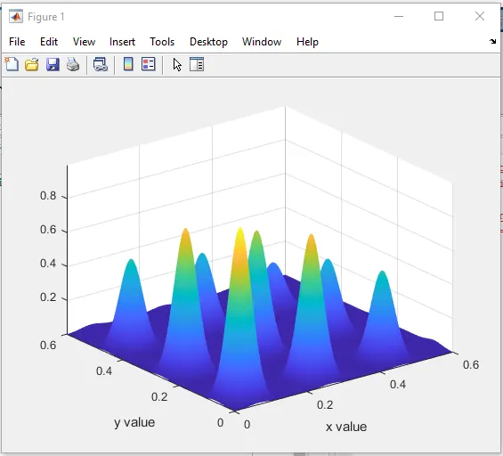
Figure 1 shows the 3D representation of stalagmite function. A function named stalagmite has been created to evaluate the mathematical expression and store the result in the form of an array. surfc(X,Y,Z) has been used to create a three-dimensional surface plot with a contour plot underneath.

Plot for unbounded inputs-

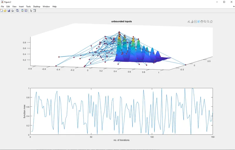
from the plot it can be observed that with the unbounded inputs ga solver is unable to calculate the global maxima. Due to random sampling the maximum value ranges between 0.1 to 1, therfore further optimization is needed.

Plot for bounded inputs-

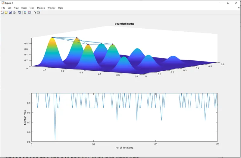
this plot shows that using the bounded inputs gets more clear result than the previous one. Here the maximum value ranges between 0.7 to 1. But still optimization is needed.

plotting bounded inputs with increased population size-

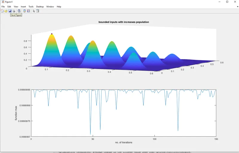
with the increased population size we get the most accurate result.

2. Explain concept of genetic algorithm in your own words and also explain the syntax for ga in MATLAB in your report.

Genetic algorithm is a search-based optimization technique. It is used to find optimal solutions to both constrained an unconstrained problems.

Genetic algorithm selects individuals form the current population to be parents and then uses them to produce the children for the next generation. By these generations the population evolves towards an optimal solution.

Initialization- After the genetic representation and the fitness function are defined, a GA proceeds to initialize a population of solutions. The population size depends on the nature of the problem, but typically contains several hundreds or thousands of possible solutions.

Selection- During each successive generation a portion of the existing population is selected to breed a new generation.

Crossover and mutation- It is the process of producing a second generation population of solutions from those selected. By producing a child solution using the methods of crossover and mutation a new solution is created which typically shares many of the characteristics of its parents and the process continues until a new population of solutions of appropriate size is generated.

Stopping Criteria of GA

MaxGenerations- The algorithm stops when the number of generations reaches max generation

MaxTime- The algorithm stops after running for an amount of time in seconds equal to maxTime

FitnessLimit- The algorith stops when the value of the fitness function for the best point in the current population is less than or equal to FitnessLimit

MaxStallGenerations- The algorithm stops when the average relative change in the fitness function value over MaxStallGeneraions is less than function tolerance.

MaxStallTime- The algorithm stops if there is no improvement in the objective function during an interval of time in seconds equal to MaxStallTime.

FunctionTolerance- The algorithm runs until the average relative change in the fitness function value over MaxStallGenerations is less than FunctionTolerance

Syntax for GA algorithm

x= ga(fun,nvars) finds a local unconstrained minimum, x, to the objective function, fun. nvars is the dimension (number of design variables) of fun.

x = ga(fun,nvars,A,b,Aeq,beq,lb,ub) defines a set of lower and upper bounds on the design variables, x, so that a solution is found in the range lb ≤ x ≤ ub. When there is no linear inequalities we set Aeq and Beq as null vector.

x = ga(fun,nvars,A,b,Aeq,beq,lb,ub,nonlcon,intcon,options) minimizes with the default optimization parameters replaced by values in options. (Set nonlcon=[] if no nonlinear constraints exist.) we Create options using optimisations.