Week 3 - Solving second order ODEs

Solving second order ODEs

objective:

is to write a program that solves the following ODE. This ODE represents the equation of motion of a simple pendulum with damping

`(d^2theta)/dt^2+b/m*(d theta)/dt+g/L*sin theta=0`

In the above equation,

g = gravity in m/s2,

L = length of the pendulum in m,

m = mass of the ball in kg,

b=damping coefficient.

Write a program in Matlab\Octave that will simulate the pendulum motion, just like the one shown in the start of this challenge.

use,

L=1 metre,

m=1 kg,

b=0.05.

g=9.81 m/s2.

Simulate the motion between 0-20 sec, for angular displacement=0,angular velocity=3 rad/sec at time t=0.

Program Code

clear all
close all
clc


% Inputs
b = 0.05;    % Damping Coefficient
g = 9.81;   % Gravity in m/s2
l = 1;      % Length of Pendulum in m
m = 1;      % Mass of the ball

% Initial Condition
theta_0 = [0;3];     %When displacement=0, velocity= 3 rad/sec

% Time Points
t_span =linspace(0,20,400); %Time array 

% Solve ODE
[t,r] = ode45(@(t,theta) ode_func(t,theta,b,g,l,m),t_span,theta_0);

% Plotting
figure(1)  
plot(t,r(:,1))
hold on
plot(t,r(:,2))
title('Motion of a Simple Damped Pendulum');
ylabel('Plot')
xlabel('Time')
legend('Displacement','Velocity')
hold off
pause(2)

% Pendulum Animation
ct=1;                     % Loop for Animation
for i=1:length(r(:,1))
x0 = 0;
y0 = 0;
x1 =l*sin(r(i,1));
y1 =-(l*cos(r(i,1)));
figure(2)
plot([-2,2],[0,0],'linewidth',5,'color','g');
hold on 
plot([x0 x1], [y0 y1],'linewidth',3,'color','black');
hold off 
hold on
plot(x1,y1,'.','markersize',50,'markerfacecolor','r','markeredgecolor','r');
hold off
title('Simulation of a Damped Pendulum Motion');
axis([-1.5 1.5 -1.5 1]);

M(ct)=getframe(gcf);
ct = ct + 1;
end

% Video of the animation
movie(M)
video=VideoWriter('Pendulum.avi','Uncompressed AVI');
open(video)
writeVideo(video,M)
close(video)

Function Code

%function program 
function [dtheta_dt] =ode_func(t,theta,b,g,l,m)
theta1= theta(1);
theta2= theta(2);
dtheta1_dt = theta2;
dtheta2_dt = -(b/m)*theta2 -(g/1)*sin(theta1);
dtheta_dt =[dtheta1_dt; dtheta2_dt];
end

Results:
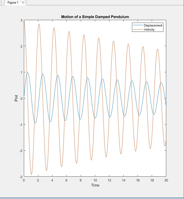
1. Graph:

2. Animation:

https://youtu.be/nsjXkutKyag

EXPLANATION:

To solve the second order diffrential equation for studying the motion of simple pendulum with damping using MATLAB.

For this first convert the second order diffrential equation into first order and then solve the equation using MATLAB.

From the ODE for the pendulum, the parameters to be considered are damping coefficient, length of the pendulum, mass of the pendulum and the acceleration due to gravity.

for a time span solution is generated. The motion of the pendulum is captured until it stops osscilating.

inputs are taken for damping coefficient, length of the pendulum, mass of the pendulum and the acceleration due to gravity.

initial condition of velocity 3 and displacement 0 is given

time space is given for 0 to 10

making use of a function ode is solved

the plotted the velocity displacement graphs.

legends and labels are given accordingly

for animation of pendulum we write the codes then

counter variable is given as 1

origin points x0 y0 defined

then x1 and y1 found using eqn

then figure 2 olotting commands are given. and labels, axis marker size, colors etc are given.

We use video M(ct)=getframe(gcf);

we are using an array, M with counter variable ct to capture the frames of the current figure.

we use an iteration for ct to capture all the frames.

Then we create a movie with the captured frames using the commands Movie, Videowriter,Videfile etc

WriteVideo command writes the craptured frames into the videofile by defining the name of the file and the compression method.