Project 2 - Rankine cycle Simulator

AIM:

Creation of Rankine cycle simulator from given input and reading the data from standard thermodynamic library of steam table.

OBJECTIVE:

1. To create a Rankine Cycle Simulator using MATLAB
2. To calculate the state points of the Rankine Cycle based on user inputs
3. To plot the T vs s and H vs s plot for the given input.

OBSERVATIONS:

The Rankine cycle is the fundamental operating cycle of all power plants where an operating fluid is continuously evaporated and condensed. The selection of operating fluid depends mainly on the available temperature range.

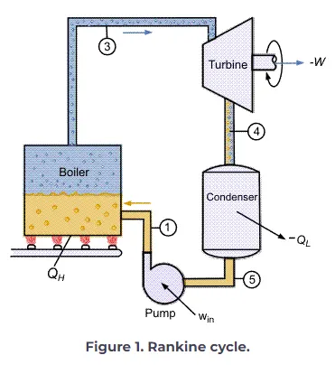
• 1-2-3 Isobaric Heat Transfer. High pressure liquid enters the boiler from the feed pump (1) and is heated to the saturation temperature (2). Further addition of energy causes evaporation of the liquid until it is fully converted to saturated steam (3).

• 3-4 Isentropic Expansion. The vapor is expanded in the turbine, thus producing work which may be converted to electricity. In practice, the expansion is limited by the temperature of the cooling medium and by the erosion of the turbine blades by liquid entrainment in the vapor stream as the process moves further into the two-phase region. Exit vapor qualities should be greater than 90%.

• 4-5 Isobaric Heat Rejection. The vapor-liquid mixture leaving the turbine (4) is condensed at low pressure, usually in a surface condenser using cooling water. In well designed and maintained condensers, the pressure of the vapor is well below atmospheric pressure, approaching the saturation pressure of the operating fluid at the cooling water temperature.

• 5-1 Isentropic Compression. The pressure of the condensate is raised in the feed pump. Because of the low specific volume of liquids, the pump work is relatively small and often neglected in thermodynamic calculations.

• 
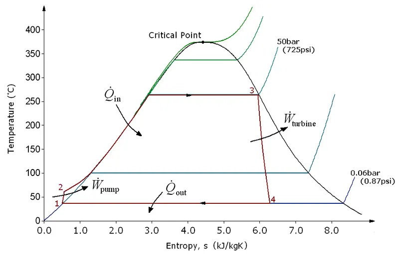
• The efficiency of the Rankine cycle is limited by the high heat of vaporization by the fluid. The fluid must be cycled through and reused constantly, therefore, water is the most practical fluid for this cycle. This is not why many power plants are located near a body of water that's for the waste heat. As the water condenses in the condenser, waste heat is given off in the form of water vapour which can be seen billowing from a plant's cooling towers. This waste heat is necessary in any thermodynamic cycle. Due to this condensation step, the pressure at the turbine outlet is lowered. This means the pump requires less work to compress the water resulting in higher overall efficiencies.

PROGRAM CODE:

clear all
close all
clc

%%
disp(' RANKINE CYCLE ');                                    % Displaying
disp('1-2 is Isentropic Expansion in the turbine');
disp('2-3 is constant pressure heat removal in the condenser');
disp('3-4 is Isentropic compression in the pump');
disp('4-1 is Constant pressure heat addition in the boiler');

%%
%Obtaining the input data
p1 = input('\nValue of pressure at turbine inlet, p1(in bar) = ');
T1 = input('\nValue of temperature at turbine inlet, T1(in degree.C) = ');
p2 = input('\nValue of temperature at condenser inlet, p2(in bar) = ');
%% 
% Extracting data _ defining variables
% State 1
h1 = XSteam('h_pT', p1, T1);        % extracting enthalpy at state pt 1
s1 = XSteam('s_pT', p1, T1);        % similarly

% State 2
s2 = s1;                            % Isentropic expansion                
sf2= XSteam('sL_p', p2);            % Saturated liquid Entropy
sg2 = XSteam('sV_p', p2);           % Saturated Vapour Entropy
x2 = (s2-sf2)/(sg2-sf2);
hf2 = XSteam('hL_p', p2);           
hg2 = XSteam('hV_p', p2);
h2 = hf2 + (x2*(hg2-hf2));

% State 3
p3 = p2;                            % Constant pressure Heat rejection in condenser
s3= XSteam('sL_p', p3);
h3 = XSteam('hL_p', p3);

% State 4
s4 = s3;
p4 = p1;
%%
% Work done by turbine
Wt = h1 - h2;

% Work done to run pump
v3 = XSteam('vL_p', p3);
Wp = v3*(p4 - p3)*100;
h4 = h3 + Wp;

%net work
Wnet = Wt - Wp;

%Heat into the system
Qin = h1 - h4;

%Heat out of the system
Qout = h2 - h3;

%Thermal efficiency
eff = (Wnet/Qin)*100;

%Specific Steam Consumption
%SSC = mass flow rate/power
SSC = (3600/Wnet);

%%
%Calculating temperatures at the state points
T3 = XSteam('Tsat_p', p3);
T2 = T3;
Cp4 = XSteam('Cp_ps', p4, s4);
Cv4 = XSteam('Cv_ps', p4, s4);
k = Cp4/Cv4;
T4 = T3/((p3/p4)^((k-1)/k));

%Calculating temperature, entropy and enthalpy at the vapour and liquid
%line for plotting
T6 = XSteam('Tsat_p', p1);
s5 = XSteam('sL_p', p1);
s6 = XSteam('sV_p', p1);
h5 = XSteam('hL_p', p1);
h6 = XSteam('hV_p', p1);
T5 = T6;

%%
%Plotting the saturation curve
T = linspace(1,375,1000);
for i = 1:length(T)

sf(i) = XSteam('sL_T', T(i));
sg(i) = XSteam('sV_T', T(i));
hf(i) = XSteam('hL_T', T(i));
hg(i) = XSteam('hV_T', T(i));
end

%Plotting T-s diagram
figure(1)
hold on
plot(sf, T, 'r','linewidth',1)
plot(sg, T, 'r','linewidth',1)
plot([s1 s2], [T1 T2], 'k', 'linewidth', 2)
plot([s2 s3], [T2 T3] ,'k', 'linewidth', 2)
plot([s3 s4], [T3 T4], 'k', 'linewidth', 2)
plot([s4 s5], [T4 T5], 'k', 'linewidth', 2)
plot([s5 s6], [T5 T6], 'k', 'linewidth', 2)
sc1 = linspace(s6, s1, 1000);
for l = 1:length(sc1)
 Tc1(l) = XSteam('T_ps', p1, sc1(l));
end
plot(sc1, Tc1, 'k', 'linewidth', 2)
text(s1+0.1, T1, '1')
text(s2+0.1, T2, '2')
text(s3, T3-20, '3')
text(s4, T4+20, '4')
title('Temp vs Entropy plot')
xlabel('Entropy ,S (Kj/kgk')
ylabel('Temperature (degree C) ')
legend('Saturation curve')


%%
%Plotting h-s diagram
figure(2)
hold on
plot(sf, hf, 'r', 'linewidth', 1)
plot(sg, hg, 'r',  'linewidth', 1)
plot([s1 s2], [h1 h2], 'k', 'linewidth', 2)
plot([s2 s3], [h2 h3], 'k', 'linewidth', 2)
plot([s3 s4], [h3 h4], 'k', 'linewidth', 2)
hc = linspace(h4, h5, 100);
for k = 1:length(hc)
sch(k) = XSteam('s_ph', p1, hc(k));
end
plot(sch,hc, 'k', 'linewidth', 2)
plot([s5 s6], [h5 h6], 'k', 'linewidth', 2)
for m = 1:length(sc1)
hc1(m) = XSteam('h_ps', p1, sc1(m));
end
plot(sc1, hc1, 'k', 'linewidth', 2)
text(s1+0.1, h1, '1')
text(s2+0.1, h2, '2')
text(s3, h3-100, '3')
text(s4, h4 +200, '4')
title('Enthalpy vs Entropy plot')
xlabel('Entropy , S (KJ/kgk) ')
ylabel('Enthalpy , H (KJ/kg)')
legend('Saturation curve','location','northwest')


%%
% Displaying Results
disp(' RESULTS');
fprintf('At State Point 1:\n');
fprintf('p1: %8.3f bar\n', p1);
fprintf('T1: %8.3f C\n', T1);
fprintf('h1: %8.3f KJ/kg\n', h1);
fprintf('s1: %8.3f KJ/kgK\n\n', s1);
fprintf('At State Point 2:\n');
fprintf('p2: %8.3f bar\n', p2);
fprintf('T2: %8.3f C\n', T2);
fprintf('h2: %8.3f kJ/kg\n', h2);
fprintf('s2: %8.3f kJ/kgK\n', s2);
fprintf('x2: %8.3f\n\n', x2);
fprintf('At State Point 3:\n');
fprintf('p3: %8.3f bar\n', p3);
fprintf('T3: %8.3f K\n', T3);
fprintf('h3: %8.3f kJ/kg\n', h3);
fprintf('s3: %8.3f kJ/kgK\n\n', s3);
fprintf('At State Point 4:\n');
fprintf('p4: %8.3f bar\n', p4);
fprintf('T4: %8.3f K\n', T4);
fprintf('h4: %8.3f KJ/kg\n', h4);
fprintf('s4: %8.3f kJ/kgK\n\n', s4);
fprintf('Turbine Work: %8.3f kJ/kg\n', Wt);
fprintf('Pump Work: %8.3f kJ/kg\n', Wp);
fprintf('Wnet: %8.3f kJ/kg\n', Wnet);
fprintf('Efficiency: %8.3f Percent \n ', eff);
fprintf('S.S.C: %8.3f kJ/kWh', SSC);

Explanation of program code:

• The creation of Rankine cycle simulator starts with some input value which are required to calculate the other state point in cycle eventually.
• The Rankine cycle process is displayed in the command window and then inputs are entered which are inlet pressure for turbine, temperature at turbine inlet and pressure at condenser.
• Then we are using XSteam function file for reading state point. First, we get the value of enthalpy and entropy at state point 1 from the XSteam function file.
• As process from 1-2 is isentropic compression the entropy at point 1 is equal to point 2. The term ‘(s_pT, p1, T1)’ refers to entropy at pressure and temperature point 1.
• The term ‘sg’ and ‘sf’ are referred to saturated liquid and saturated vapor entropy respectively. This value is used to calculate other function according to mathematical relations.
• Similarly, other points are taken from XSteam function file which are necessary to calculate other parameters. After that work done in turbine and pump are calculated for further getting the net work done Rankine cycle.
• After calculating the net work done the efficiency of the Rankine cycle is calculated along with specific steam consumption which is steam consumed by a locomotive cylinders per unit of output of work done.
• Then temperature at each point of cycle is calculated using input taken from start of the program and data taken from XSteam file. For given temperature range from lower to higher entropy points are calculated to create the T-S plot. Similarly, another for loop is used to create the saturation curve in each plot.
• Then plotting is done respectively for T-s and H-s graph in Rankine cycle and each state point value has been put in command window.

RESULT:

Inference of Plot:

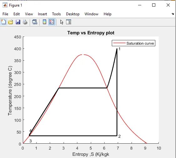
From the above diagram as we can see along the saturation curve point 1 start with turbine from which heat rejection is started which is again isentropic process. The steam is get cooled in condenser and in form of saturated liquid as it is under the curve. Then it was pumped to enter in boiler where its temperature is increased to change it from saturated liquid to saturated vapor form.

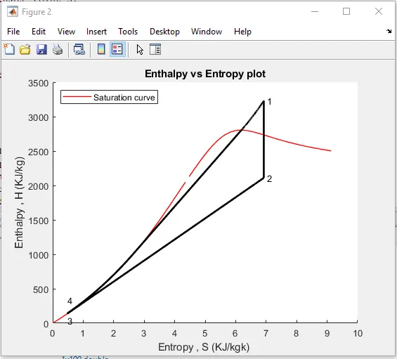
As we can see from above plot the steam entropy changes during the process with respect to enthalpy. As the heat added in the system the entropy has been increased and similarly as the heat removed from the system the entropy drops with similar rates.

State points of the Rankine Cycle based on user inputs:

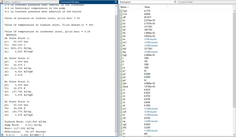
Conclusion:

We have created the Rankine cycle simulator for the given input, in which we have taken the data from XSteam function file. And the Rankine cycle plots have generated by calculating the state points, efficiency and the output is printed in the command window.