Week 4.1 - Genetic Algorithm
Aim - To optimize the stalagmite function using genetic algorithm techniques using Matlab.
To understand the genetic algorithm first, we need to understand the following concepts to build a basic understanding of the genetic algorithm.
1) what is optimization? and discussing various optimization techniques?
let us first understand that what optimization is, and various techniques in optimization.
optimization-
Optimization is the process of making something better(such as a design, system, or decision) as fully perfect, functional, or effective as possible, this also helps us to find the best possible results under a set of constraints. This process is executed again and again till the final result or the output is satisfactory. This includes maximizing the product, strength, reliability, efficiency, and utilization.
Various optimization techniques that can be used to optimize the result.
Deterministic method:
In this method, the output of the model is fully determined by the parameter of the initial conditions. This uses specific rules from moving from one solution to another. let us understand with the help of an example:
stress analysis of wing is determined as the output result(stress value) is totally dependent on the initial condition (loading condition) and the parameters like material and forces acting on the component.
Stochastic method:
This method is used for minimizing and maximizing an objective function, this possesses some inherent randomness, it is a probabilistic approach. This method is gaining popularity due to some properties which deterministic method does not possess. Let us understand with an example imagine a company that provides energy to households. This company is responsible for delivering energy to households based on how much they demand. Typically, this problem could be solved as a simpler Linear Program (LP) with constraints based on demand from households. Though this is convenient, the future demand of households is not always known and is likely dependent on factors such as the weather and time of year. Therefore, there is uncertainty and our basic LP model will not suffice. Stochastic programming offers a solution to this issue by eliminating uncertainty and characterizing it using probability distributions.
The following is the procedure followed by an optimization process.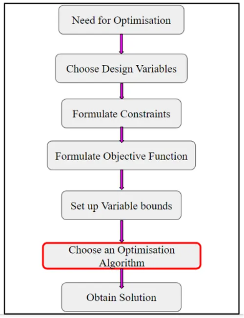
Variables - Variable is a process that may vary during optimization is my variables. an Example is the dimension of a design that can be scale-up or vary to get minimum stress.
Constraints - During the optimization your output must not go beyond certain limits are known as constraints. An example one can reduce the material in such a way that the stress must not exit the ultimate stress of the material.
Objective function- This can be predicted by the mathematical model that includes all the variables as input. for example z = (x,y) here the z output is totally dependent on the input variable (x,y).
variable bound- These are the range of the variable input, that will be varied at every iteration to provide an optimized result.for example, the design variable can be varied in between the set of a range to get the minimum stress.
2) what is a genetic algorithm?
The concept of Genetic Algorithm
A genetic algorithm is a natural process that is used for the selection of the fittest individuals. The main use of the genetic algorithm is for reproduction to produce offspring of the next generation, this process of selecting and reproducing the fittest individual is inspired by Charles Darwin’s and named it the "Theory of evolution".
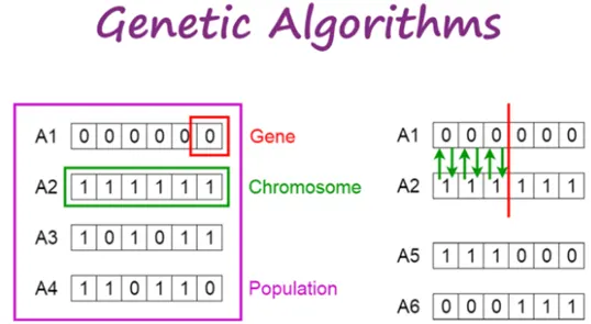

The process of natural selection starts with the selection of the fittest individuals from a population. They produce offspring which inherit the characteristics of the parents and will be added to the next generation. If parents have better fitness, their offspring will be better than parents and have a better chance at surviving. This process keeps on iterating and in the end, a generation with the fittest individuals will be found.
Five phases are considered in a genetic algorithm. They are
Initial population
Fitness function
Selection
Crossover
Mutation
3) How genetic algorithms work? Where the genetic algorithm is used?
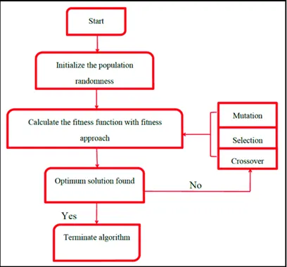
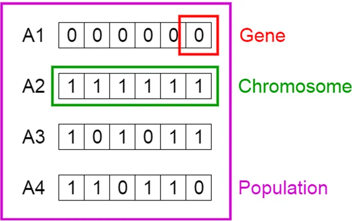
Initial Population- the process begins with a set of individuals which is called a Population. An individual is characterized by a set of parameters (variables) known as Genes. Genes are joined into a string to form a Chromosome (solution).
What is fitness function? to determine the fitness function we are comparing how fittest an individual is, basically we are comparing the individuals with one another. It gives a fitness score to each individual and based on the fitness score the individual will be selected for reproduction.
Selection -The idea of the selection phase is to select the fittest individuals and let them pass their genes to the next generation. Here, two pairs of individuals are selected according to their fitness score, higher will be the fitness the more chance is for the selection for reproduction.
cross over - cross over is a process of taking two-parents' solutions and producing a child from them. For each pair of parents to be mated, a crossover point is chosen at random from within the genes.
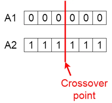
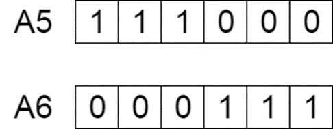
Offspring are created by exchanging the genes of parents among themselves until the crossover point is reached. 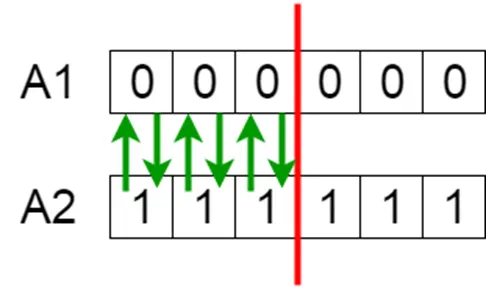
now the new offsprings are added to the population.
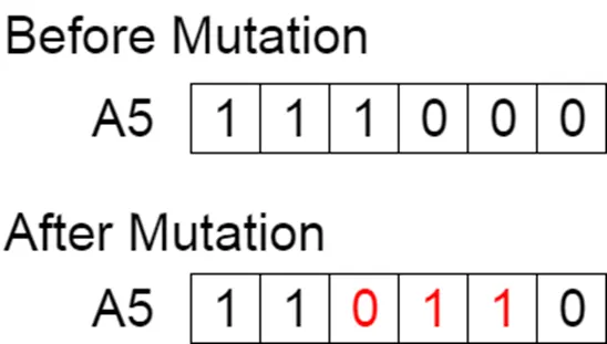
Mutation- Mutation is used to carry out the genetic diversity from one generation of the population of chromosomes to the next generation. This mutation process is too important to perform because if it is not performed then the chromosomes will be too similar to each other. The mutation occurs to maintain diversity within the population and prevent premature convergence and results in local minima.
Advantages of GAs
GAs have various advantages that have made them immensely popular. These include −
Does not require any derivative information (which may not be available for many real-world problems).
Has very good parallel capabilities.
Optimizes both continuous and discrete functions and also multi-objective problems.
Provides a list of “good” solutions and not just a single solution.
Useful when the search space is very large and there are a large number of parameters involved.
Always provide good results over time.
Limitations of GAs
If not implemented properly, the GA may not converge to the optimal solution.
Where there is simple problem and for that the derivative values is known then this is not suited i.e genetic algorithm
Main code:
clear all
close all
clc
%Defining our search space
x =linspace(0,.6,150);
y =linspace(0,.6,150);
num_case=60;
%creating a 2D mesh
[xx,yy]= meshgrid(x,y);

%evaluating the stalagmite function
for i=1:length(xx);
    for j =1:length(yy);
input_vector(1)=xx(i,j);
input_vector(2)=yy(i,j);
f(i,j)= stalagmite(input_vector);
    end
end

tic
 for k = 1:num_case;
     [inp,fval(k)] = ga(@stalagmite,2);
     x_1(k) = inp(1);
     y_1(k) = inp(2);
 end
study1_time=toc

figure (1)
hold on
grid on
surfc(xx,yy,-f)
shading interp
title('stalagmite plot')
xlabel ('X')
ylabel('Y')

figure(2)
subplot(2,1,1)
surfc(xx,yy,-f)
shading interp
hold on
plot3(x_1,y_1,-fval,'marker','o','markersize',5,'markerfacecolor','g')
title('unbounded inputs')
subplot(2,1,2)
plot(-fval)
xlabel('iterations')
ylabel('function minimum')

% 2nd case study  statistical behavior
tic
for s = 1:num_case;
    [input,fval(s)]= ga(@stalagmite,2,[],[],[],[],[0,0],[0.6,0.6]);
    x_2(s)= input(1);
    y_2(s)= input(2);

end
study2_time = toc
figure(3)
subplot(2,1,1)
surfc(xx,yy,-f)
shading interp
hold on
plot3(x_2,y_2,-fval,'marker','o','markersize',5,'markerfacecolor','g')
title('unbounded inputs')
subplot(2,1,2)
plot(-fval)
xlabel('iterations')
ylabel('function minimum')


% 3rd case study  increasing ga iterations
options = optimoptions('ga');
options = optimoptions(options,'populationsize',150);
tic
for m = 1:num_case;
    [input,fval(m)]= ga(@stalagmite,2,[],[],[],[],[0,0],[.6,.6],[],[],options);
    x_3(m)= input(1);
    y_3(m)= input(2);

end
study3_time = toc
figure(4)
subplot(2,1,1)
surfc(xx,yy,-f)
shading interp
hold on
plot3(x_3,y_3,-fval,'marker','o','markersize',5,'markerfacecolor','g')
title('unbounded inputs')
subplot(2,1,2)
plot(-fval)
xlabel('iterations')
ylabel('function minimum')
Function code:
function [f] = stalagmite(input)
x = input(1);
y = input(2);
f1x = (sin(5.1*pi*x + 0.5))^6;
f1y = (sin(5.1*pi*y + 0.5))^6;
f2x = exp((-2.7726)*(x-(0.0667))^2/0.64);
f2y = exp((-2.7726)*(y-(0.0667))^2/0.64);

f = -(f1x*f1y*f2x*f2y);
end
Exaplanation:
- The code starts with defining x and y as inputs using linspace
- A function known as Stalagmite_func is defined as hown in the 2nd stage of codes.
- 2 for loops are incorporated in the main code so that all the combinations of x and y values is taken in the stalagmite_func function
- In the 1st study GA function runs for 80 iterations. Plots of the stalagmites and maximum values generated in each iteration is shown.
- In the 2nd study GA function is incorporated with lower and upper bounds and runs for 80 iterations. Plots of the stalagmites and maximum values generated in each iteration is shown.
- In the 3rd study GA function is incorporated with lower and upper bounds along with the population size of 200. Plots of the stalagmites and maximum values generated in each iteration is shown.
Result:
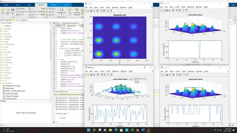
Study 1:
Stalagmite basic:
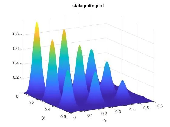
as we can see that there are more up-growing peaks, basically are my stalagmite structure. However, the function tends to give the negative value which gives the local minima's, so to make the function positive for getting the local and global maxima's. (upgrowing peaks). The highest peak is called global maxima and others are local maxima's.
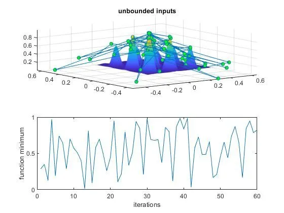
In the first study there are no lower and upper limits hence the GA does not the search space is between 0 and 1. Hence each time the program is executed different optimum values are are obtained as shown in the plot 2.
Study-2:
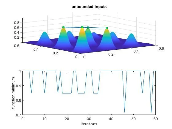
Here we can observe lower and upper limits are included in the GA. Hence most of the maximum values obtained in each iteration varies between (1) and (0.6). This method narrows down the maximum values to 4 points as shown in the plot 1.
Study-3:
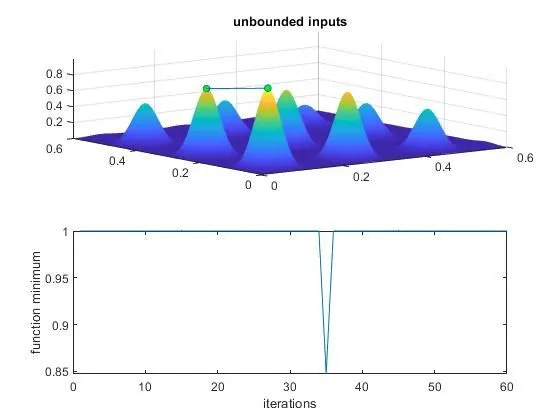
The resulted line from high peak to low peak is the critical point for my global maxima and the time taken by it is 36.4559 which is approx 3 times greater than the case study one. As the population size is large enough to carry out 50 iterations at the same time. however, we got our optimum maximized solution.
Conclusion:
Optimised stagalmite function and global maxima of function is found successfully by using MATLAB.
References:
https://skill-lync.com/knowledgebase/genetic-algorithm-explained