Week 3 - Solving second order ODEs

Aim:

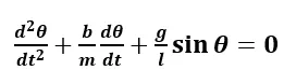
• Write the program to simulate the Pendulum motion for the given motion equation
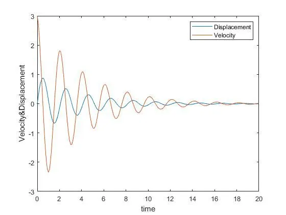
• Plot the graft between Displacement&Velocity to time.
• Simulate the motion between 0-20 sec, for angular displacement=0, angular velocity=3 rad/sec at time t=0.When you do this you will get the position of the pendulum as a function of time. Use this information to animate the motion of the pendulum, as shown in the Assignment.

Theory:

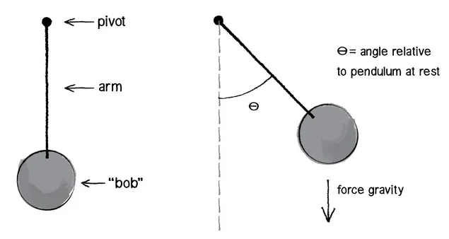
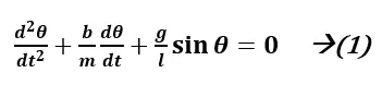
Here b = Damping Co-efficient

m = mass

g = Gravity

l = Length of pendulum

Let us consider

θ = θ₁ ---->(a)

dθ₁/dt = θ_{2 ----->}(b)

dθ₁/dt = [(-b/m) θ₂]-[(g/l)sin θ₁] ---->(c)

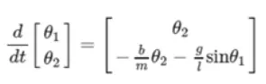
From using (a) and (b) we form matrix eqution

ODE Function Code:

function[dtheta_dt] = ode_func(t,theta,b,g,l,m)
 theta1=theta(1);
 theta2=theta(2);
 dtheta1_dt = theta2;
 dtheta2_dt = -(b/m)*theta2 - (g/l)*sin(theta1);
 dtheta_dt = [dtheta1_dt;dtheta2_dt];
end

Explanation:

• In this we are converting the given ODE equation into two different equations.
• The two equations are later computed and assigned to single matrix.

ODE Code:

close all
clear all
clc

%Static inputs given in he problem
b=0.05;
g=9.81;
l=1;
m=0.1;

%intial condition
theta_0 = [0;3];

%time points
t_span = linspace(0,20,200);

%Solving the ODE Function
[t,result] = ode45(@(t,theta) ode_func(t,theta,b,g,l,m), t_span, theta_0);

%ploting Velocity and displacement
figure(1)
plot(t,result(:,1))
hold on
plot(t,result(:,2))
xlabel('time')
ylabel('Velocity&Displacement')
legend('Displacement','Velocity')
ang=result(:,1);
%count command for iteration
t=1;
%loop to generate all the slides to pendulum simulation
for i=1:length(ang)
    omega=ang(i);
    figure(2)
    %fixed coordinates
    x0 = 0;
    y0 = 0;
    %moving coordinates of the bob
    x1=l*cos((3*pi/2)+omega);
    y1=l*sin((3*pi/2)+omega);
    %Plotting the bob motion
    plot([x0 x1],[y0 y1],'linewidth',3);
    hold on;
    plot(x1,y1,'o','markers',15,'markerFaceColor','k');
    hold on;
    plot([-2 2],[0 0],'linewidth',6);
    hold off;
    axis([-2 2 -2 2])
    grid on
    pause(0.2)
    M(t)=getframe(gcf);
    t=t+1;
end

%To create a animation of the simple pendulum
movie(M)
videofile = VideoWriter('Motion_of_Simple_Pendulum.avi','uncompressed AVi');
open(videofile)
writeVideo(videofile,M)
close(videofile)
    
    

Explanation:

• Give the inputs “b=0.02, g=9.81, l=1, m=0.1”which are given in the problem.
• Input the initial ‘θ’ conditions and Time span of the operation.
• Call the ode_func using ode45 inbuild function of the MATLAB.
• Plot the plot between the velocity & displacement to the Time.
• For Generating the required slides for the animation of Simple pendulum motion, we are using for loop.
• We assign the each frame of the pendulum motion to each element of the matrix M.
• We Generate the Video Clip of the Pendulum motion using Movie Command.

Result:

Plot:

Animation of Simple Pendulum:https://youtu.be/881uw7kgvKU