Week 4.1 - Genetic Algorithm
AIM
Write a code in MATLAB to optimise the stalagmite function and find the global maxima of the function.
THEORY
- optimization
it is a field of study which deals with maximizing or minimizing of a function subject to different input parameters.
2.stalagmite mathematical model
it is a mathematical model used to find the local maxima or local minima using genetic algoritham .ga is explained in detail below.
3. Genetic algoritham
- ga is an optimization technique which is used to solve non-linear ,non-differential optimization problem
- it is based of mechanics of natural selection and natural genetics so called survival of fittest proposed by "Charles Darwin".
- it starts with an initial generation of candidate solution that are tested against an objective function
- subsequent generations evolve from 1st through selection ,cross over&mutation,
- these process is explained in detail below
selection: In this, we are selecting the best performing bit strings from one generation to the next generation. i.e based on the Fitness.
Let, take an example
here we have 2 parents who have good performance so selecting them, based on the fitness.

Crossover: Due to they performed well, therefore taking common between them to create a child as shown below.
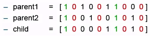
Mutation: Taking parent and mutate certain variable and create a child based on mutation. i.e in mutation, we are adding other qualities to the child.

syntax of ga
ga function is used to minimize a function hence inorder to maximize we inverse the function .
Syntax
x = ga(fun,nvars)
x = ga(fun,nvars,A,b)
x = ga(fun,nvars,A,b,Aeq,beq)
x = ga(fun,nvars,A,b,Aeq,beq,lb,ub)
x = ga(fun,nvars,A,b,Aeq,beq,lb,ub,nonlcon)
x = ga(fun,nvars,A,b,Aeq,beq,lb,ub,nonlcon,options)
x = ga(fun,nvars,A,b,Aeq,beq,lb,ub,nonlcon,intcon)
x = ga(fun,nvars,A,b,Aeq,beq,lb,ub,nonlcon,intcon,options)
x = ga(problem)
[x,fval] = ga(___)
[x,fval,exitflag,output] = ga(___)
[x,fval,exitflag,output,population,scores] = ga(___)
EXPLANATION
x= ga(fun,nvars,A,b)xtofun, subject to the linear inequalitiesA*x≤b.gaevaluates the matrix productA*xas ifxis transposed (A*x').x= ga(fun,nvars,A,b,Aeq,beq)xtofun, subject to the linear equalitiesAeq*x=beqandA*x≤b. (SetA=[]andb=[]if no linear inequalities exist.)gaevaluates the matrix productAeq*xas ifxis transposed (Aeq*x').x= ga(fun,nvars,A,b,Aeq,beq,lb,ub)x, so that a solution is found in the rangelb≤x≤ub. (SetAeq=[]andbeq=[]if no linear equalities exist.)x= ga(fun,nvars,A,b,Aeq,beq,lb,ub,nonlcon)nonlcon. The functionnonlconacceptsxand returns vectorsCandCeq, representing the nonlinear inequalities and equalities respectively.gaminimizes thefunsuch thatC(x)≤0andCeq(x) = 0. (Setlb=[]andub=[]if no bounds exist.)x= ga(fun,nvars,A,b,Aeq,beq,lb,ub,nonlcon,options)options. (Setnonlcon=[]if no nonlinear constraints exist.) Createoptionsusingoptimoptions.x= ga(fun,nvars,A,b,[],[],lb,ub,nonlcon,IntCon)x= ga(fun,nvars,A,b,[],[],lb,ub,nonlcon,IntCon,options)IntContake integer values.
STALAGMITE FUNCTION
function[f]=stalagmite(input_vector)
x=input_vector(1);
y=input_vector(2);
f1_x=(sin((5.1*pi*x)+0.5))^6;
f1_y=(sin((5.1*pi*y)+0.5))^6;
f2_x=exp(-4*log(2).*(((x-0.0667).^2)/0.64));
f2_y=exp(-4*log(2).*(((y-0.0667).^2)/0.64));
f=-(f1_x.*f1_y.*f2_x.*f2_y);
end
study-1: (statistical behavior)
clear all
close all
clc

% program for study 1
% defining array
x=linspace(0,0.6,150);
y=linspace(0,0.6,150);
[xx,yy]=meshgrid(x,y);
num_cases=150;

for i=1:length(xx)
for j = 1:length(yy)
    input_vector(1)=xx(i,j);
    input_vector(2)=yy(i,j);
    f(i,j)= stalagmite(input_vector);
end
end
% 1st study _statistical behavior
tic
for i= 1:num_cases
    [inputs,fopt(i)]=ga(@stalagmite,2);
    xopt(i)=inputs(1);
    yopt(i)=inputs(2);
end
study1_time =toc
fopt=-fopt;
figure(1)
subplot(2,1,1)
hold on
surfc(x,y,-f)
shading interp
plot3(xopt,yopt,fopt,'marker','o','MarkerSize',6,'MarkerFaceColor','r')
title('unbounded inputs')
subplot(2,1,2)
plot(fopt)
xlabel('iterations')
ylabel('function maximum')
EXPLANATION OF CODE
- x,y are 1_D arrays created using linspace command
- it is converted into 2-D using meshgrid command
- num_cases=150 is a command used to run the ga code 150 times
- then ga function is called and a no of variables is passed as input which is equal to 2 and storing x,yand f_opt value which function produced
- tik and toc command is used to find the time it takes to measure study
- new figure window is opened
- subplot is created (creates multiple plots in same figure window)
- 1st plot is surfc(x,y,f),plot 3 command is used for plotting x,y,ga_opt,which helps us to know how the algoritham perfoms
- second subplot in which directly optimum value is plotted as a function of iterations is create
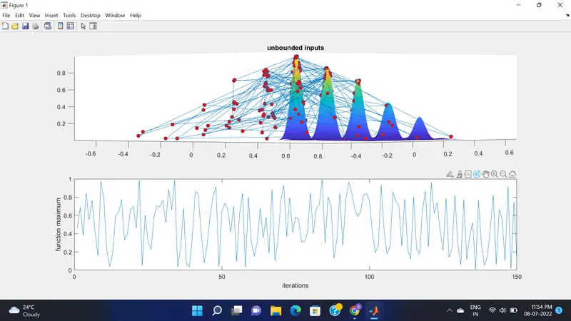
figure-1
RESULT
we get multiple results due to random sampling and maximum value varies from 0.2 to 0.8 . time taken for 1st study is 4.12735seconds .hence further optimization is requiered
study-2: (statistical behavior with upper and lower bounds)
[0,0]=upper and lower bound for x
[1,1]=upper and lower bound for y
clear all
close all
clc

% program for study 2
% defining array
x=linspace(0,0.6,150);
y=linspace(0,0.6,150);
[xx,yy]=meshgrid(x,y);
num_cases=150;

for i=1:length(xx)
for j = 1:length(yy)
    input_vector(1)=xx(i,j);
    input_vector(2)=yy(i,j);
    f(i,j)= stalagmite(input_vector);
end
end

%study 2 with upper and lower bounds
tic
for i=1:num_cases
    [inputs,fopt(i)]=ga(@stalagmite,2,[],[],[],[],[0;0],[1;1]);
    xopt(i)=inputs(1);
    yopt(i)=inputs(2);
end
fopt=-fopt;
study2_time=toc
figure(2)
subplot(2,1,1)
hold on
surfc(x,y,-f)
shading interp
title('BOUNDED INPUTS')
xlabel('x values')
ylabel('y values')
plot3(xopt,yopt,fopt,'marker','o','MarkerSize',6,'MarkerFaceColor','r')
subplot(2,1,2)
plot(fopt)
xlabel('iterations')
ylabel('function maximum')
EXPLANATION
Here the only difference in program is along with ga function we set a upper bound and lower bound
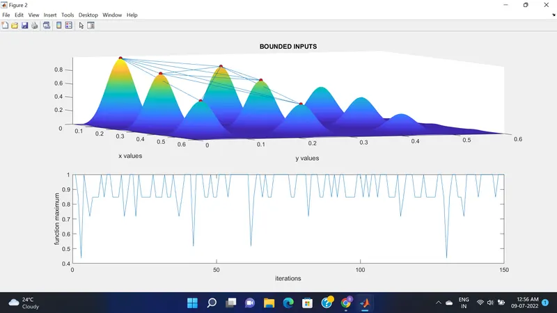
figure -2
RESULT
now our results are more clear and the maximum range is between 0.7 to0.85.time taken for study=5.50825 seconds .still optimization is needed
STUDY-3 : (increasing no of iterations)
clear all
close all
clc

% program for study 1
% defining array
x=linspace(0,0.6,150);
y=linspace(0,0.6,150);
[xx,yy]=meshgrid(x,y);
num_cases=150;

for i=1:length(xx)
for j = 1:length(yy)
    input_vector(1)=xx(i,j);
    input_vector(2)=yy(i,j);
    f(i,j)= stalagmite(input_vector);
end
end
% study 3 increasing GA iterations
options=optimoptions('ga');
options=optimoptions(options,'PopulationSize',500);

tic
for i=1:num_cases
    [inputs,fopt(i)]=ga(@stalagmite,2,[],[],[],[],[0,0],[0.6,0.6],[],[],options)
    xopt(i)=inputs(1);
    yopt(i)=inputs(2);
end
fopt=-fopt;
study3_time=toc
figure(3)
subplot(2,1,1)
hold on
surfc(x,y,-f)
shading interp
title('increased iterations')
xlabel('x values')
ylabel('y values')
plot3(xopt,yopt,fopt,'Marker','o','MarkerSize',6,'MarkerFaceColor','r')
subplot(2,1,2)
plot(fopt)
xlabel('iterations')
ylabel('funtion maximum')
EXPLANATION
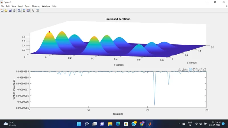
To optimize the results & getting more accuracy we increase the iteration in genetic algorithm.By default it takes 50 values .In this study we increase the population size becuase if population size is too small it will not calculate global maxima and minima instead it will calculate local max and min .By using options command we set population size to 500
figure-3
RESULT
now we get the most accurate result between 0.999999985-0.99999998.
time taken for study 3= 31.275 seconds
COMBINED STUDIES PROGRAM
clear all
close all
clc

% program for study 1
% defining array
x=linspace(0,0.6,150);
y=linspace(0,0.6,150);
[xx,yy]=meshgrid(x,y);
num_cases=150;

for i=1:length(xx)
for j = 1:length(yy)
    input_vector(1)=xx(i,j);
    input_vector(2)=yy(i,j);
    f(i,j)= stalagmite(input_vector);
end
end
% 1st study _statistical behavior
tic
for i= 1:num_cases
    [inputs,fopt(i)]=ga(@stalagmite,2);
    xopt(i)=inputs(1);
    yopt(i)=inputs(2);
end
study1_time =toc;
fopt=-fopt;
figure(1)
subplot(2,1,1)
hold on
surfc(x,y,-f)
shading interp
plot3(xopt,yopt,fopt,'marker','o','MarkerSize',6,'MarkerFaceColor','r')
title('unbounded inputs')
subplot(2,1,2)
plot(fopt)
xlabel('iterations')
ylabel('function maximum')

%study 2 with upper and lower bounds
tic
for i=1:num_cases
    [inputs,fopt(i)]=ga(@stalagmite,2,[],[],[],[],[0;0],[1;1]);
    xopt(i)=inputs(1);
    yopt(i)=inputs(2);
end
fopt=-fopt;
study2_time=toc
figure(2)
subplot(2,1,1)
hold on
surfc(x,y,-f)
shading interp
title('BOUNDED INPUTS')
xlabel('x values')
ylabel('y values')
plot3(xopt,yopt,fopt,'marker','o','MarkerSize',6,'MarkerFaceColor','r')
subplot(2,1,2)
plot(fopt)
xlabel('iterations')
ylabel('function maximum')

% study 3 increasing GA iterations
options=optimoptions('ga');
options=optimoptions(options,'PopulationSize',500);

tic
for i=1:num_cases
    [inputs,fopt(i)]=ga(@stalagmite,2,[],[],[],[],[0,0],[0.6,0.6],[],[],options)
    xopt(i)=inputs(1);
    yopt(i)=inputs(2);
end
fopt=-fopt;
study3_time=toc
figure(3)
subplot(2,1,1)
hold on
surfc(x,y,-f)
shading interp
title('increased iterations')
xlabel('x values')
ylabel('y values')
plot3(xopt,yopt,fopt,'Marker','o','MarkerSize',6,'MarkerFaceColor','r')
subplot(2,1,2)
plot(fopt)
xlabel('iterations')
ylabel('funtion maximum')

max_value=fopt
RESULT
to get maximum value of the program we are using the function max_value=fopt and we get max value as 1.0000
CONCLUSION
1)Hence, we are able to optimise the stalagmite function and find the global maxima of the function.
2)The (ga) is only used for the minimum function therefore to Maximize the function we inversed the minimum function.
ERRORS FACED
ERROR 1: @ function not used infront of ga , error cleared by using @ga

apart from this no major errors occured .
REFERENCES
https://www.mathworks.com/discovery/genetic-algorithm.html https://en.wikipedia.org/wiki/Genetic_algorithm