Project 2 - Rankine cycle Simulator

AIM

1. To Simulate a Rankine cycle using matlab.
2. Extracting Steam and water properties from XSteam data (IAPWS IF - 97 standard)
3. Calculating all the state points of the cycle based on User inputs.
4. Plotting the T vs s and H vs s plot for the given input.

THEORY

A Rankine cycle is an ideal thermodynamic cycle which uses heat energy to produce mechanical work which is then converted into electrical energy .

The working process is very simple a fuel is used to produce heat energy in Boiler using the heat energy water is used a medium to produce steam which is then expanded onto a Turbine to produce mechanical work.

It is an idealized cycle hence losses are neglected

Process and working

• Process 1-2 - Isentropic expansion in the turbine
• process 2-3- Constant pressure heat Heat rejection in condenser
• process 3-4- Isentropic compression in the pump
• Process 4-1- Constant pressure heat addition in the boiler

• process 1-2 - the dry satuarated vapour expands through the turbine generating power .This decreases the temparature and pressure of the vapour and some condensation may occur
• process 2-3 - The vapour liquid mixture leaving the turbine is condensed at low pressure usually in a surface condenser using cooling water.
• process 3-4 - The pressure of the condensate is raised in the feed pump because of the low specific volume of liquids,the pump work is relatively small and often neglected in thermodynamic calculations
• process 4-1 -High pressure liquid enters the boiler from feed pump and is heated to the satuaration temparature .further addition of energy causes evapouration of the liquid until it is fully converted to saturated steam

PROGRAM

% Rankine cycle simulator 
fprintf('rankine cycle\n');
fprintf('1-2 is ISENTROPIC EXPANSION\n')
fprintf('2-3 is CONSTANT PRESSURE HEAT REMOVAL\n');
fprintf('3-4 ISENTROPIC COMPRESSION\n');
fprintf('4-1 CONSTANT PRESSURE HEAT ADDITION\n');

% defining inputs 
p1=30;  % turbine inlet pressure
t1=400; % turbine inlet temparature
p2=0.05; % condenser inlet pressure 

% taking data from xsteam for state point 1 
h1=xsteam('h_pt',p1,t1);
s1=xsteam('s_pt',p1,t1);

% state variables at point 2 
s2=s1;
sf2=xsteam('sL_p',p2);
sg2=xsteam('sV_p',p2);
x2=(s2-sf2)/(sg2-sf2);
hf2=xsteam('hl_p',p2);
hg2=xsteam('hV_p',p2);
h2=hf2+(x2*(hg2-hf2));

% state variables at point 3

p3=p2;
s3=xsteam('sL_p',p3);
h3=xsteam('hL_p',p3);

% state variables at point 4
s4=s3;
p4=p1;

% work done by turbine 
w_t=h1-h2;

% work done by pump 
v3=xsteam('vL_p',p3);
w_p=v3*(p4-p3)*100;
h4=h3-w_p;

% net work done for rankine cycle 
w_net=w_t-w_p;

% heat addition to system 
Q_in=h1-h4;

% heat rejected from system
Q_out=h2-h3;

% Thermal efficency of rankine cycle 
T_eff=(w_net/Q_in)*100;

% specific steam consumption (mass flow rate /net work done)
sp_s=(3600/w_net);

% calculation of temparature at all state point 2,3,4 
t3= xsteam('Tsat_p',p3);
t2=t3;
cp4=xsteam('cp_ps',p4,s4);
cv4=xsteam('Cv_ps',p4,s4);
k=(cp4/cv4);
t4=t3/((p3/p4)^((k-1)/k));

% calculation of other constants for saturated liquid and vapour 
t6=xsteam('Tsat_p',p1);
s5=xsteam('sL_p',p1);
s6=xsteam('sV_p',p1);
h5= xsteam('hL_p',p1);
h6=xsteam('hV_p',p1);
t5=t6;

% plotting 
T= linspace(1,560,1000);
for i=1:length(T)
    sf(i)=xsteam('sL_T',T(i));
    sg(i)=xsteam('sV_T',T(i));
    hf(i)=xsteam('hL_T',T(i));
    hg(i)=xsteam('hV_T',T(i));
end

% plotting T-S diagram for Rankine cycle 
figure(1)
hold on 
plot(sf,T,'color','b','LineWidth',2)
plot(sg,T,'color','b','LineWidth',2)
plot([s1 s2],[t1 t2],'Color','r','LineWidth',3)

plot([s2 s3],[t2 t3],'Color','r','LineWidth',3)

plot([s3 s4],[t3 t4],'Color','r','LineWidth',3)
plot([s4 s5],[t4 t5],'Color','r','LineWidth',3)
plot([s5 s6],[t5 t6],'Color','r','LineWidth',3)

s_1=linspace(s6,s1,1000);
for j=1:length(s_1)
    Tc(j)=xsteam('T_ps',p1,s_1(j));
end

plot(s_1,Tc,'Color','r','linewidth',3)
text(s1+0.1,t1,'1')
text(s2+0.1,t2,'2')
text(s3,t3-20,'3')
text(s4,t4+20,'4')
title('TEMPARATURE VS ENTROPY')
xlabel('Entropy(kj/kg-k)')
ylabel('Temparature(0c)')
legend('satuaration curve')


% plotting H-S diagram for Rankine cycle 
figure(2)
hold on 
plot (sf,hf,'Color','b','LineWidth',2)
plot(sg,hg,'Color','b','LineWidth',2)
plot([s1 s2],[h1 h2],'Color','r','linewidth',3)
plot([s2 s3],[h2 h3],'Color','r','linewidth',3)
plot([s3 s4],[h3 h4],'Color','r','linewidth',3)
hc=linspace(h4,h5,100);
for k= 1: length(hc)
    s_c(k)=xsteam('s_ph',p1,hc(k));
end
plot(s_c,hc,'color','r','linewidth',3)
plot([s5 s6],[h5 h6],'Color','r','linewidth',3)
for l= 1: length(s_1)
    h_c(1)=xsteam('h_ps',p1,s_1(l));
end

plot([s5 s6],[h5 h6],'Color','r','LineWidth',3)
for l=1:length(s_1)
    h_c(1)=xsteam('h_ps',p1,s_1(1));
end
 
plot(s_1,h_c,'Color','r','LineWidth',3)
text(s1+0.1,h1,'1')
text(s2+0.1,h2,'2')
text(s3,h3-100,'3')
text(s4,h4+200,'4')
title('Enthalpy vs Entropy')
xlabel('Entropy(kj/kg-k)')
ylabel('Enthalpy (kj/kg)')
legend('saturation curve')

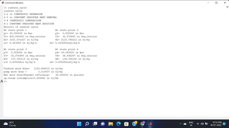
% Displaying results in command window 

disp('Results of rankine cycle')
fprintf('At state point 1\t\t\t\t\t')
fprintf('At state point 2\n')
fprintf('p1=%10f in Bar\t\t\t\t',p1);
fprintf('p2=%10f in Bar\n',p2);
fprintf('T1=%11f in Deg.celcius\t\t',t1);
fprintf('T2=%11f in Deg.celcius\n',t2);
fprintf('H1=%12f in kj/kg\t\t\t',h1);
fprintf('H2=%12f in kj/kg\n',h2);
fprintf('s1=%9f in kj/kg-k\t\t\t',s1);
fprintf('s2=%9finkj/kg-k\n',s2);

fprintf('\n')
fprintf('At state point 3\t\t\t\t\t')
fprintf('At state point 4\n')
fprintf('p3=%10f in Bar\t\t\t\t',p3);
fprintf('p4=%10f in Bar\n',p4);
fprintf('T3=%11f in Deg.celcius\t\t',t3);
fprintf('T4=%11f in Deg.celcius\n',t4);
fprintf('H3=%12f in kj/kg\t\t\t',h3);
fprintf('H4=%12f in kj/kg\n',h4);
fprintf('s3=%9fin kj/kg-k\t\t\t',s3);
fprintf('s4=%9finkj/kg-k\n',s4);
fprintf('\n')
fprintf('Turbine work done=%14f in kj/kg\n',w_t);
fprintf('pump work done = %15f in kj/kg\n',w_p);
fprintf('Net work done=%17 in kj/kg\n',w_net);
fprintf('Thermal efficency=%13f in percent\n',T_eff);
fprintf('sp.steam consumption=%f in kj/kw\n',sp_s);

EXPLANATION OF THE PROGRAM

• in step 1 fprintf is used to print different sates in a Rankine cycle
• in step 2 inputs like pressure and temparature are defined
• x steam is used to extract steam and water properties like enthalpy ,entropy,at specific pressure and temparature for saturated liquid, saturated vapour conditions etc
• at state point-1 input pressure is taken in bars ,at state point one inlet temparature is taken in degree celcius ,temp at condenser inlet at state 2 is in degree celcius
• using x steam we calculate state variables at point 1,2,3,4
• h1=xsteam(h_pt,p1,t1) this input return value of enthalpy of water at a pressure p1 and temparature t1
• The net work ,work done by turbine ,work done to run the pump,heat in ,heat out are calculated using standard thermodynamic relation
• efficency and specific steam consumption of the rankine cycle is calculated
• T,s and h are extracted at vapour and liquid line for plotting ,after 4th point for the variation you observe in the plot .
• saturation curve is plotted in red for saturated liquid and satuarated gas
• plot of T vs s and T vs h are created from all points obtained in the program

PLOTS

figure 1 (Temparature vs Entropy)

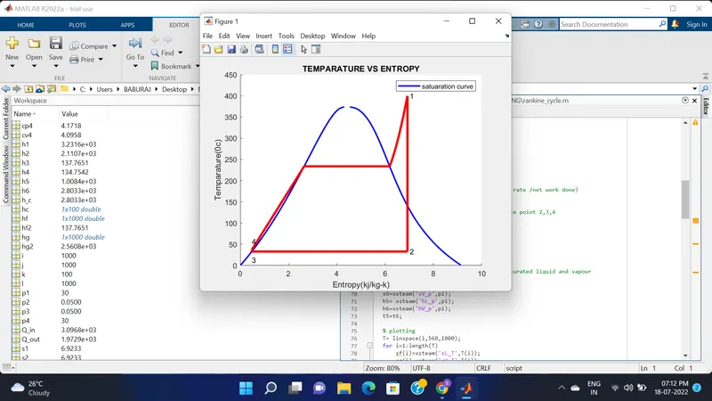
figure 2 (Enthalpy vs Entropy)

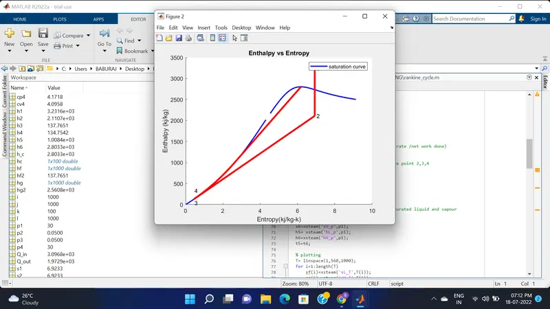
figure 3 ( Results shown in command window )

ERRORS FACED

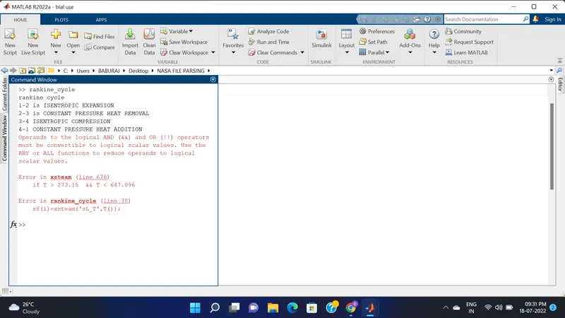
error occured due to improper using of alphabet in for loop ,apart from this no major errors was formed

REFERENCES

https://en.wikipedia.org/wiki/Rankine_cycle

https://energyeducation.ca/encyclopedia/Rankine_cycle