Week 4.1 - Genetic Algorithm

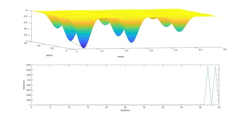
Aim : To optimise the stalagmite function and find the global maxima of the function.

Genetic algorithm(GA): A natural selection process that micmics the biological evolution, used for solving optimisation problems with both bounded and unbounded constrains.

GA iterates modifying a polpulation of induvidual solutions, selecting individuals from the current poplulation and using them as parents for the next generation.

Genetic algorithm syntax :

x= ga(@func, nvars)

where func is the fucntion name and nvars is the number of variables

x= ga(@func,nvars,A,B,)

where A and B are linear ineqaulities

x = ga(@func,nvars,A,B,Aeq,Beq,lb,ub,nonlcon,intcon,options)

where A,B = linear inequality constraints

Aeq,Beq = linear eulity constraints

lb = lower bound

up = upper bound

nonlcon = non-linear constraints

intcon = vector of positive intergers

options = optimisation options

close all
clear all
clc

%creating search space
x = linspace(0,0.6,600);
y = linspace(0,0.6,600);

%mesh creating
[X,Y] = meshgrid(x,y);

% ga runs 50 times
num_cases = 50;
%stalagmite function evaluation
for i = 1:length(X)
    for j = 1:length(Y)
        input_vector(1) = X(i,j);
        input_vector(2)= Y(i,j);
        %calling function 
        f(i,j) = stalagmitefunc(input_vector);
    end 
end

surf(X,Y,f)
shading interp
xlabel('xaxsis');
ylabel('yaxsis');

tic

% study 1 
for i = 1:num_cases
    [inputs,fopt(i)] = ga(@stalagmitefunc,2);
    xopt(i) = inputs(1);
    yopt(i) = inputs(2);
end

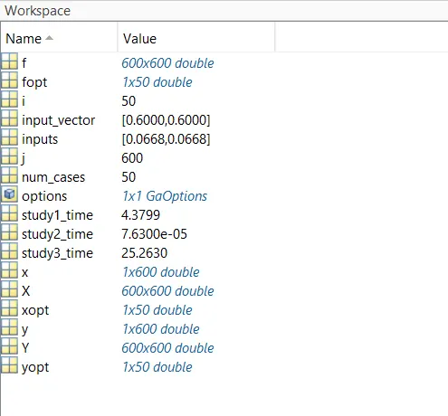
study1_time = toc;

figure(1)
subplot(2,1,1);
hold on
surf(x,y,f);
shading interp
plot3(xopt,yopt,fopt,'marker','o','markersize',5,'markerfacecolor','c')
xlabel('xaxsis');
ylabel('yaxsis');
subplot(2,1,2);
plot(fopt)
xlabel('iterations');
ylabel('minimum');

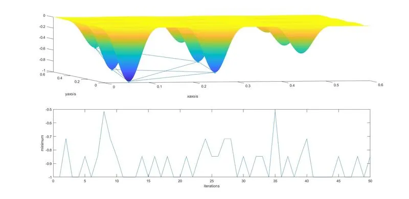
% study 2 with upper bound(up) and lower bound(lp)
for i = 1:num_cases
    [inputs,fopt(i)] = ga(@stalagmitefunc,2,[],[],[],[],[0;0],[1;1]);
    xopt(i) = inputs(1);
    yopt(i) = inputs(2);
end

tic
study2_time = toc;

figure(2)
subplot(2,1,1);
hold on
surf(x,y,f);
shading interp
plot3(xopt,yopt,fopt,'marker','o','markersize',5,'markerfacecolor','c')
xlabel('xaxsis');
ylabel('yaxsis');
subplot(2,1,2);
plot(fopt)
xlabel('iterations');
ylabel('minimum');

% study 3 with optimisation options
options = optimoptions('ga');
options = optimoptions(options,'Populationsize',300)

for i = 1:num_cases
    [inputs,fopt(i)] = ga(@stalagmitefunc,2,[],[],[],[],[0:0],[1:1],[],[],options);
    xopt(i) = inputs(1);
    yopt(i) = inputs(2);
end

study3_time = toc;

figure(3)
subplot(2,1,1);
hold on
surf(x,y,f);
shading interp
plot3(xopt,yopt,fopt,'marker','o','markersize',5,'markerfacecolor','c')
xlabel('xaxsis');
ylabel('yaxsis');
subplot(2,1,2);
plot(fopt)
xlabel('iterations');
ylabel('minimum');

%stalagmite function 
function f = stalagmitefunc(input_vector)

x = input_vector(1);
y = input_vector(2);


f1 = (sin(5.1*pi*x+0.5))^6;
f2 = (sin(5.1*pi*y+0.5))^6;
f3 = exp((-4*log(2)*(x-0.0667)^2)/0.64);
f4 = exp((-4*log(2)*(y-0.0667)^2)/0.64);

[f] = -(f1*f2*f3*f4);