Week 3 - Solving second order ODEs

close all
clear all 
clc

%input values 
b = 0.02;
m = 0.1;
g = 9.81;
l = 0.75;
%intial comditions
theta_0 = [0,3];
% time span
t_span = linspace(0,20,100);

%solving ode
[t,results] = ode45(@(t,theta) ode_pendulum(t,theta,b,g,l,m),t_span,theta_0);

%plotting the result 
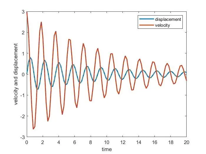
plot(t,results,'linewidth',2)
hold on 
plot(t,results,'--')
xlabel('time')
ylabel('velocity and displacement')
legend('displacement','velocity')
theta = results(:,1);

%creating animation using plot command 
ct = 1
for i = 1:length(theta)
    angle = theta(i);
    figure(2)
    title('simple pendulumn')
    x0 = 0;
    y0 = 0;
    x1 = l*cos(3*pi/2+angle);
    y1 = l*sin(3*pi/2+angle);
    plot([x0,x1],[y0,y1],'linewidth',2)
    hold on
    plot(x1,y1,'o','markers',20)
    hold on
    plot([-3,3],[0,0],'linewidth',3)
    hold off
    axis([-5,5,-2,2])
    pause(0.02)
    M(ct) = getframe(gcf)
   ct = ct+1;
end
    %writing and saving the animation file 
  movie(M)
  videofile = VideoWriter('simplependulumn.avi','Uncompressed AVI');
  open(videofile)
  writeVideo(videofile,M)
  close(videofile)

Function code

function [dtheta_dt] = ode_pendulum(t,theta,b,g,l,m)
theta1 = theta(1);
theta2 = theta(2);
dtheta1_dt = theta2;
dtheta2_dt = -b/m*theta2-g/l*sin(theta1);
dtheta_dt = [dtheta1_dt;dtheta2_dt];
end

the code starts from defining the input values such as damping coefficient(b) , mass (m), length(l), gravitational accelration(g).

the initial displacement and initial velocity are defined as theta_o = (0,3)

using the inbuilt ode45 solver we can solve only first order differentials, so we created a system of two first order differential equations. The output was recieveds as [t,results],

t - time and results inculde displacement and velocuty for a particular time intervel.

Animation file link - https://youtu.be/GuRcgGLSCC4