Week 4.1 - Genetic Algorithm
DEFFINE:
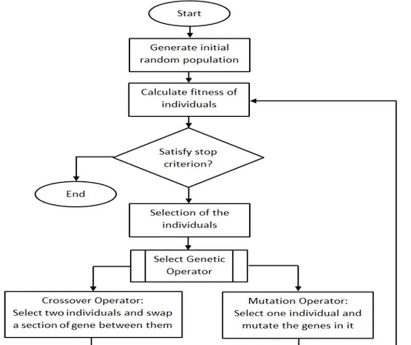
* The genetic algoritham works on the process of natural selecation where the fittest individuals are selected for reproducation in order produced offspring of the next generation .
AIM:
* To study about genetic algoritham and to calculate the global maxima of stalagmite function using genetic algoritham
OBJECTIVE:
* To study about the genetic algorithim and stalagmite function .to plot graphs based on the studies done for genetic algorthim
THEORY:
* The algoritham begins by creating a random initial population of individual selections and it keeps on modyfing the population repetadely creating sequence of new popuation .the algoritham uses the individuals in the generation to create the next population
* Selecation rules select the individuals called parents that contribute to the population at the generation
* Crossover rules combine two parents to form children for the next generation
* Mutation rules apply random changes to individual parents to form children
THE FOWCHART :
WHAT is a stalagmite function :
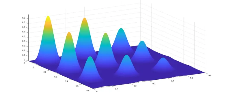
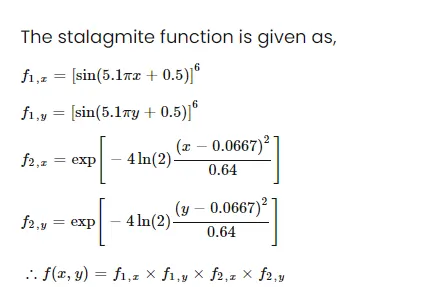
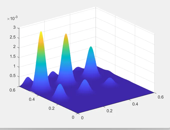
* Stalagmite function is a mathematical model which helps to generate local minima and maxima .it is a three dimensional function and way the function is designed is that it has a lot of local maxima or minima and one glopal maxima or minima .the name stalagmite is acutelly a type of rock formation that arises from the floor of a cave due to accumulation of material deposited on the floor from ceiling drippings .
syntax for defining 'ga'(genetic algoritham)-matlab:
* The 'ga' syntax in matlab is used to find the minimum function using ga .there are several ways to define the 'ga' function depending on the proplem being solved
. x=ga(fun,nvars)
x=optimal solution
fun=objective function
nvars=number of variables
. x=ga(fun,nvars,A,B,Aeq,Beq,lb,ub)
A,B= linear inequality constraints
Aeq,Beq=linear equality constraints
. x=ga(fun,nvars,A,B,Aeq,Beq,lb,up,nonlcon,intcon,options)
nonlcon=Nonlinear constraints
intcon=integer values
options=optimization options
CODING:
function [f] = stalagmite(input_vector)

a=input_vector(1);
b=input_vector(2);


term1=(sin((5.1*pi*a)+0.5))^6;
term2=exp(-4*log(2)*((a-0.0667)^2)/0.64);
term3=(sin((5.1*pi*b)+0.5))^6;
term4=exp(-4)*log(2)*((b-0.0667)^2)/0.64;


[f]=-(term1*term2*term3*term4);  %inverts the objective function
end
clear all
close all
clc
% Defining our search space
x = linspace(0,0.6,150);
y = linspace(0,0.6,150);
% Creating a 2Dimensional mesh
[xx,yy] = meshgrid(x,y);
% Evaluating the stalagmite function
for i = 1:length(xx)
for j = 1:length(yy)
input_vector(1)=xx(i,j);
input_vector(2)=yy(i,j);
f(i,j) = stalagmite(input_vector);
end
end
surfc(xx,yy,-f)
shading interp
[x,fval] = ga(@stalagmite,2)
clear all
close all
clc

x = linspace(0,1,150);
y = linspace(0,1,150);
[xx,yy] = meshgrid(x,y);

% Evaluating the stalagmite function
for i = 1:length(xx)
    for j = 1:length(yy)
        input_vector(1)=xx(i,j);
        input_vector(2)=yy(i,j);
        f(i,j) = stalagmite(input_vector);
    end
end
surfc(xx,yy,-f)
shading interp
tic
% study 1-stalagmite behavior
num_cases = 50;
for i = 1:num_cases
    [inputs,fopt(i)] = ga(@stalagmite,2);
    xopt(i) = inputs(1);
    yopt(i) = inputs(2);
end

study1_time = toc

figure(1)
subplot(2,1,1)
surfc(xx,yy,-f)
hold on
shading interp
plot3(xopt,yopt,-fopt,'Marker','o','MarkerSize',5,'MarkerFaceColor','r')
title('unbounded inputs')
subplot(2,1,2)
plot(-fopt)
xlabel('Iterations')
ylabel('function minimum')

tic
% study 2-statistical behavior -with upper and lower bounds
for i = 1:num_cases
    [inputs,fopt(i)] = ga(@stalagmite,2,[],[],[],[],[0;0],[1;1]);
    xopt(i) = inputs(1);
    yopt(i) = inputs(2);
end
study2_time = toc

figure(2)
subplot(2,1,1)
surfc(xx,yy,-f)
hold on
shading interp
plot3(xopt,yopt,-fopt,'Marker','o','MarkerSize',5,'MarkerFaceColor','r')
title('Bounded inputs')
subplot(2,1,2)
plot(-fopt)
xlabel('Iterations')
ylabel('Function minimum')

% study 3 increasing GA iterations
options = optimoptions('ga')
options = optimoptions(options,'PopulationSize', 150);


tic
for i = 1:num_cases
    [inputs,fopt(i)] = ga(@stalagmite,2,[],[],[],[],[0;0],[1;1],[],options);
    xopt(i) = inputs(1);
    yopt(i) = inputs(2);
end
study3_time = toc
figure(3)
subplot(2,1,1)
hold on
surfc(x,y,-f)
shading interp
plot3(xopt,yopt,fopt,'Marker','o','MarkerSize',5,'MarkerFaceColor','r')
subplot(2,1,2)
plot(-fopt)
xlabel('No. of Iterations')
ylabel('function maximum')
CODING EXPLANATION:
* Clear all
*close all
*clc
* Then' X' array and 'Y' array is defining using 'linspace' command to creat value at 150 equal intervals
* A 2D mesh of x and y array is creating by using 'mesh grid 'command and the number of iterations or cases that the code should perform is defined
* To evaluate the stalagmite function for loop is used where 'i' is intialzied and for every where of 'i' another 'for' loop is used initilize
* The inpu vector values 'xx' 'yy' are defined as stalagmite function for these input vector is defined this will form basic stalagmite function and we can plot its separetly if needed
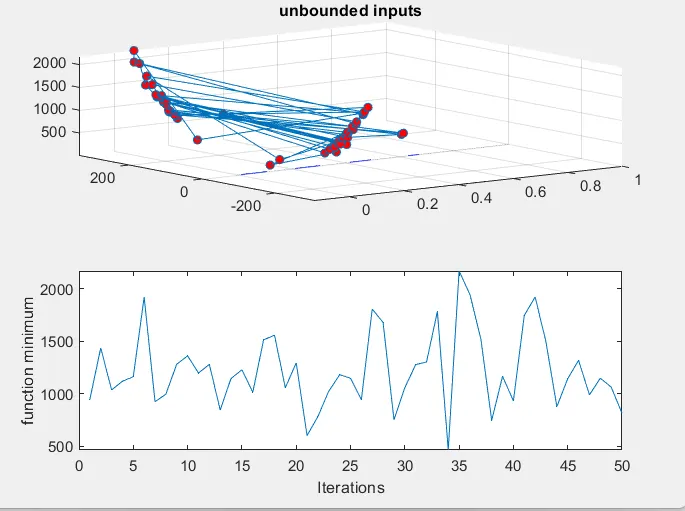
* After preparing the inputs needed for the function ,next step is to obtain the results for 3 cases of genetic algorthim .in first case or study ,the maximum value of function is founded out with no restrications ,no bound and no limts
* This is done using 'for' loop where we use 'ga' syntax to given values for inputs and optimum max value .the stalagmite function is called 'ga' syntax and number of variables 'nvars' are 2
* To known the time that is taken to solve the loop for 50 iterations ,'tic' and 'toc' command is used before and ofter the loop respectively
* Then function created in the loop is plotted by using 'surfc' command for 'xx,yy and function output'.To neglect the gridlines on the surface and obtain a smooth and clean plot ,'shading interp' command is used .the 'subplot' (2,1,1) is used a plots multiple plots on same figure which also divides figure in grid of 2*1 and axes to placed at 1
RESULTS:
STUDY 1-Statistical Behaviour
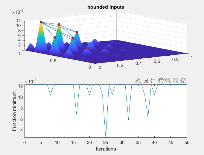
STUDY 2-Statistical behaviour with upper and lower bounds
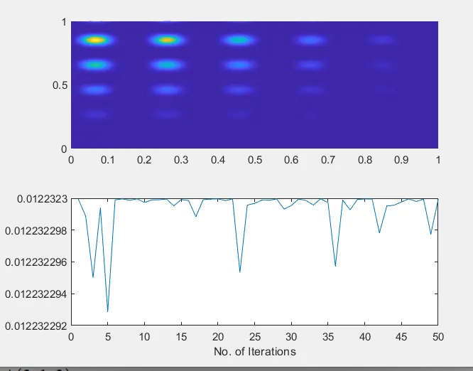
STUDY 3 -Statistical behaviour with increasing iterations
STUDY 4-
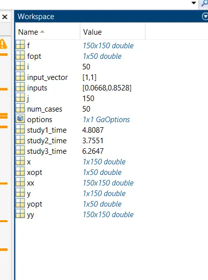
WORKPLACE: