Week 3 - Solving second order ODEs

AIM:

         * To solve the ODE which represents the equation of motion a simple pendulum with damping 

OBJECTVE:

          * To write a program that solve the following ODE which represents equation of motion of simple pendulum with damping and create an animation video of output by solving ODE 

      THEORY:

                * Ordinary differential equation (ODE) -is a differential equation containing one or more functions of one independent variable and the derivatives of those functions .the term ordinary is used in contrast with the term partial differential equation which may be with respect to more than one independent variables 

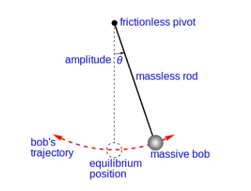
                * simple pendulum - the pendulum is an idealzied mathematical model of a pendulum this is weight on the end of massless cord suspension from a pivot without frication .when given an initial push it will swing back and forth at a constant amplitude.

   GOVERING EQUATIONS :

            

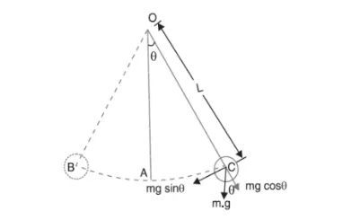
          'theta' is angle made by the movable link with vertica axis 

         L is length of movable rod

         m is the mass of bob ,b is damping coefficient of the system 

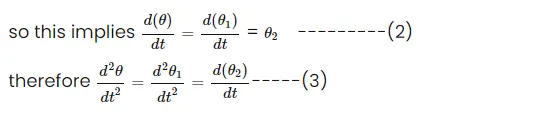
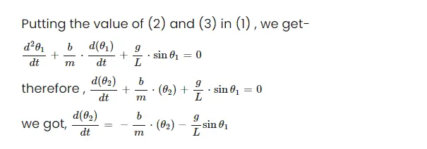
     To solve this ODE we need to reduce the order of equation into lower order 

                 'theta' = 'theta'1

  

INPUT:

        * L = 1 meter 

        * m = 1kg

        * b = 0.05

        * g = 9.81 m/s^2

        * time span = 0-20 sec 

        * angular displacement = 0

        * angular velocity = 3 rad /sec 2 at time t= 0

CODING:

clear all
close all
clc


b=0.05;
g=9.81;
l=1;
m=0.1;

% initial condition
theta_0 = [0;5];

% time points
t_span = linspace(0,20,500);
% solve ODE
[t, results] = ode45(@(t,theta) ode_func(t, theta, b,g,l,m),t_span, theta_0);
figure(1)
plot(t,results(:,1))
hold on
plot(t,results(:,2))
ylabel('plot')
xlabel('time')

% creating animation of the pendulum
ct = 1;
theta_1 = results(:,1);

for i = 1:length(results(:,1))

   % initial co-ordinates
    x_start = 0;
    y_start = 0;
    theta_2 = theta_1(i);

    % final co-ordinates
    x_end = 1*sin(theta_2);
    y_end = -1*cos(theta_2);


    % ploting for animation 
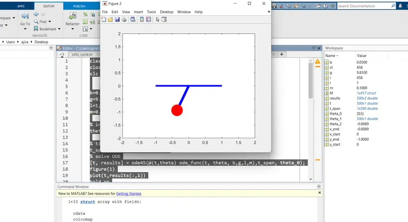
    figure(2)
    % base of pendulum
    plot([-1,1],[0,0],'LineWidth',4,'Color','b')
    hold on
    % starting of pendulum
    line([x_start x_end],[y_start y_end],'linewidth',6,'color','b')
    hold on
    % bob of pendulum
    plot(x_end,y_end,'Marker','o','MarkerSize',28,'MarkerFaceColor','r')
    axis([-2 2 -2 2])
    pause(0.03)
    hold off 
    M(ct) = getframe(gcf)
    ct = ct+1;
end 

  % creating movie from captured frames 
  movie(M)
  videofile = VideoWriter('simple_pendulum.avi','Uncompressed AVI');
  open(videofile);
  writeVideo(videofile,M);
  close(videofile);

CODE FOR FUNCTION PROGRAM:

               function [dtheta_dt] = ode_func(t,theta,b,g,l,m)

                        theta1 = theta(1)

                        theta2 = theta(2)

                         dtheta1_dt = theta2;

                       dtheta2_dt = -(b/m)*theta2-(g/l)*sin(theta1);

                     dtheta_dt = [dtheta1_dt: dtheta2_dt];

end

CODE EXPLANATION:

               1) In the first step input and initial condition of a simple pendulum 

               2) Then the program is written to solve the ode in which matlab inbuilt function (ode45) is used with constant theta and another function used which define seperatly in function program 

   OUTPUT:

                

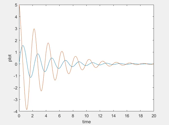
WORKSPACE:

      

 

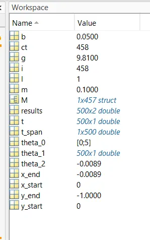
The pendulum starts oscillating  in a inverter direction in animated video

 

https://drive.google.com/file/d/1iRLlUFm_0hZjBmmjt3Y6_4ba8BhsFecV/view?usp=sharing