Week 4.1 - Genetic Algorithm
Aim- Write a code in MATLAB to optimize the stalagmite function and find the global maxima of the function
Optimization-optimization is decision making process it helps to find the best results
G.A.(Genetic Algorithm)=genetic algorithm is biological term,it makes better & better product from one generation to next generation two concepts included under genetic algorithm 1) crossover 2)mutation
1)crossover =one child is simillar with two parents
2)mutation =child totally different from parents
G.A.(Genetic Algorithm)-Genetic Algorithm is a search based optimization technic based on the principles of genetic and natural selection it is frequently used to final optimal or near optimal solutions
it is frequently used to solve optimization problems in research and in machine learning
To find 150 values between 0 to 0.6 using linspace command
Explanation=To find 150 values between 0 to 0.6 using linspace command
3)num cases=50 Explanation=Genetic algorithm runs 50 times
4)[xx,yy]=meshgrid(x,y)Explanation= to convert x,y 1Dimensions into 2Dimensions xx,yy
%Evaluting the stalagmite functions
5) for i=1:length(xx)Explanation='i' value access the xx array values
for j=1:length(yy)Explanation='j' value access the yy array values
input_vector(1)=xx(i,j);
input_vector(2)=yy(i,j)
f(i,j)=stalagmite('input vector')Explanation=input vector is 2 column,stalagmite is a function use for the calculating f value
end
end
Explanation=This entire for loop use for generating data for plot earlier
6)surfc(xx,yy,-f)Explanation=surfc command create 3d plot using xx,yy-2D Dimensions & '-f ' use for global maxima
7)tic= Explanation=start stopwatch timer & toc=read elapsed time from stopwatch timer;
%stastical behaviour
8)for i=1:num_cases Explanation= Genetic algorithm runs 50 times
[inputs,fopt(i)]=ga(@stalagmite,2); Explanation=ga=genetic algorithm ,stalagmite=function ,2=no of variables input,fopt(i)=optimum value of function predict
xopt(i)=inputs(1)
yopt(i)=inputs(2)
end
Explanation-it's loop use for calculating x opt value & y opt value
9)study time=toc = read elapsed stopwatch timer
figure(1)
10)subplot(2,1,1)=subplot (m,n,p)divides the current figure into an m-by-n grid and creates axis in the position specified by p MATLAB numbers subplot position by row.the first subplot is the first column of the row , the second subplot
is the second column of the first row and so on if axes exist in the specified position then this command makes the axes is the current axes
%study 2-stastical behaviour with upper & lower bounds
11)tic=Explanation=start stopwatch timer & toc=read elapsed time from stopwatch timer;
12)for i=1:num cases Explanation=Genetic algorithm runs 50 times
[inputs,fopt(i)]=ga (@stalagmite,2,[],[],[],[],[0;0],[0.6;0.6]);=Defines a set of lower & upper bounds on the design variables x,so that a solution is found the range 1b_< x _
xopt(i)=inputs(i)
yopt(i)=inputs(2)
end
Explanation -this entire loop sets stastical behaviour of upper &lower bounds to reduces maximum solution value
13)study2 time =toc; Explanation= read elapsed stopwatch timer
figure (2)
14)subplot(2,1,1)Explanationsubplot (m,n,p)divides the current figure into an m-by-n grid and creates axis in the position specified by p MATLAB numbers subplot position by row.the first subplot is the first column of the row , the second subplot is the second column of the first row and so on if axes exist in the specified position then this command makes the axes is the current axis
15)xlabel('iteration') Explanation =no of performance of ga algorithms cycle
16)ylabel('functions maximum')=showing y axis value of ga algorithms value
hold on
17)surfc(xx,yy,-f)Explanation=surfc command create 3d plot using xx,yy-2D Dimensions & '-f ' use for global maxima
18)shading interp (to reduces grid on the stalgamite)
19)plot3(xopt,yopt,-fopt,'marker','o','markerSize,'5''markerfacecolor','r')
title ('bounded inputs')
20)subplot(2,1,2) subplot(2,1,1)Explanationsubplot (m,n,p)divides the current figure into an m-by-n grid and creates axis in the position specified by p MATLAB numbers subplot position by row.the first subplot is the first column of the row , the second subplot is the second column of the first row and so on if axes exist in the specified position then this command makes the axes is the current axes
21)xlabel('iteration') Explanation =no of performance of ga algorithms cycle
22)ylabel('functions maximum')=showing y axis value of ga algorithms value
%study 3 increase ga iteration
23)Options =Optimoptions ('ga ,'populationsize',170);Options=optimoptions (solvername,name,value) returns options with specified parameters set using one or more name value pair argument
24)Optimoptions=minimizes with the default optimization parameters replaced by values in options (set non coln=[] )if no non linear constraints exist create options using optmoptions
25) for i=1:num_cases
[inputs,fopt(i)]=ga(@stalagmite,2,[],[],[],[],[0;0],[0.6;0.6],[],[],options);
xopt(i)=inputs(1)
yopt(i)=inputs(2);
end
Explanation -this entire loop sets stastical behaviour of upper &lower bounds to reduces maximum solution value
26)study2 time =toc; Explanation= read elapsed stopwatch timer
figure (3)
27)subplot(2,1,1)Explanationsubplot (m,n,p)divides the current figure into an m-by-n grid and creates axis in the position specified by p MATLAB numbers subplot position by row.the first subplot is the first column of the row , the second subplot is the second column of the first row and so on if axes exist in the specified position then this command makes the axes is the current axis
hold on
28)surfc(xx,yy,-f)Explanation=surfc command create 3d plot using xx,yy-2D Dimensions & '-f ' use for global maxima
29)shading interp (to reduces grid on the stalgamite)
29)plot3(xopt,yopt,-fopt,'marker','o','markerSize,'5''markerfacecolor','r')
title ('bounded inputs')
30)subplot(2,1,2) subplot(2,1,1)Explanationsubplot (m,n,p)divides the current figure into an m-by-n grid and creates axis in the position specified by p MATLAB numbers subplot position by row.the first subplot is the first column of the row , the second subplot is the second column of the first row and so on if axes exist in the specified position then this command makes the axes is the current axes
31)xlabel('iteration') Explanation =no of performance of ga algorithms cycle
32)ylabel('functions minimnum')=showing y axis value of ga algorithms value
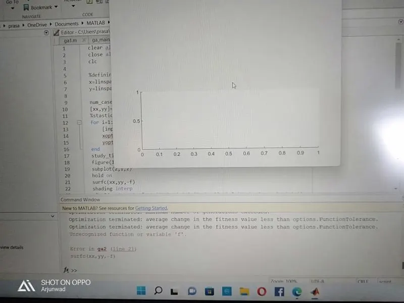
eror =forgetting calculate 'f' value & applying plot3(-fopt) solution= to calculating 'f' value using for loop (i,j)&xx,yy & type comman plot3=f(-opt)
clear all
close all
clc
%defining our search space
x=linspace(0,0.6,150);
y=linspace(0,0.6,150);
num_cases=50;
[xx,yy]=meshgrid(x,y);
%Evaluting the stalagmite function
for i=1:length(xx)
for j=1:length(yy)
input_vector(1)=xx(i,j);
input_vector(2)=yy(i,j);
f(i,j)=stalagmite(input_vector);
end
end
surf(xx,yy,-f)
shading interp
tic
%stastical behaviour
for i=1:num_cases
[inputs,fopt(i)]=ga(@stalagmite,2);
xopt(i)=inputs(1);
yopt(i)=inputs(2);
end
study_time=toc;
figure(1)
subplot(2,1,2)
hold on
surfc(xx,yy,-f)
shading interp
plot3(xopt,yopt,-fopt,'Marker','o','MarkerSize',5,'MarkerFacecolor','r')
title('unbounded inputs')
subplot(2,1,1)
plot(-fopt)
xlabel('iteration')
ylabel('function maximum')
%study2_stastical behaviour with upper & lower bounds
tic
for i=1:num_cases
[inputs,fopt(i)]=ga(@ stalagmite,2,[],[],[],[],[0;0],[0.6;0.6]);
xopt(i)=inputs(1);
yopt(i)=inputs(2);
end
study2_time=toc;
figure(2)
subplot(2,1,1)
hold on
surfc(xx,yy,-f)
shading interp
plot3(xopt,yopt,-fopt,'marker','o','MarkerSize',5,'MarkerFaceColor','r')
title('bounded inputs')
subplot(2,1,2)
plot(-fopt)
xlabel('iterations')
ylabel('functions maximum')
%study 3 increaseing GA Iterations
options=optimoptions('ga','PopulationSize',170);
for i=1:num_cases
[inputs,fopt(i)]=ga(@stalagmite,2,[],[],[],[],[0;0],[0.6;0.6],[],[],options);
xopt(i)=inputs(1);
yopt(i)=inputs(2);
end
study3_time=toc;
figure(3)
subplot(2,1,1)
hold on
surfc(xx,yy,-f)
shading interp
plot3(xopt,yopt,-fopt,'marker','o','markersize',5,'markerfacecolor','r')
title('bounded inputs')
subplot(2,1,2)
plot(-fopt)
xlabel('iterations')
ylabel('function maximum')
function[f]=stalagmite(input_vector)
fx=(sin(5.1*pi*input_vector(1)+0.5))^6;
fy=(sin(5.1*pi*input_vector(2)+0.5))^6;
fxx=exp((-4*log(2)*(((input_vector(1)-0.667)^2)/0.64)));
fyy=exp((-4*log(2)*(((input_vector(2)-0.667)^2)/0.64)));
f=-(fx*fy*fxx*fyy);
end