Week 4.1 - Genetic Algorithm

%stalagmite function

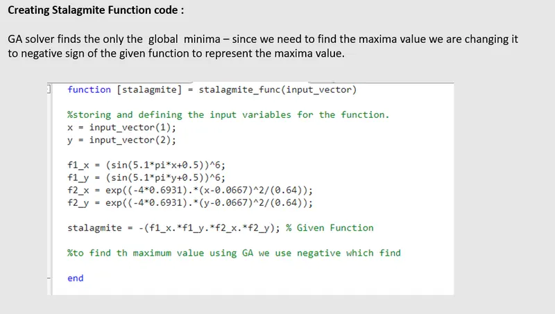
function [stalagmite] = stalagmite_func(input_vector)

%storing and defining the input variables for the function.
x = input_vector(1);
y = input_vector(2);

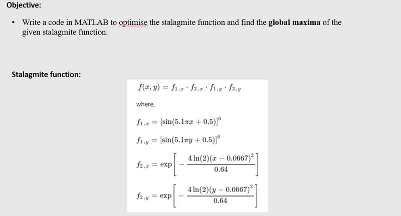
f1_x = (sin(5.1*pi*x+0.5))^6;
f1_y = (sin(5.1*pi*y+0.5))^6;
f2_x = exp((-4*0.6931).*(x-0.0667)^2/(0.64));
f2_y = exp((-4*0.6931).*(y-0.0667)^2/(0.64));

stalagmite = -(f1_x.*f1_y.*f2_x.*f2_y); % Given Function

%to find th maximum value using GA we use negative which find

end

%Matlab code 

close all
clear all

%defining search space

x = linspace(0,0.6,150);
y = linspace(0,0.6,150);

%creating a 2-Dimensional Mesh

[xx,yy] = meshgrid(x,y);

%Evaluate  the stalgamatie function

for i = 1:length(xx)
   for j= 1:length(yy)

   input_vector(1) = xx(i,j);
   input_vector(2) = yy(i,j);
   
f(i,j) = stalagmite_func(input_vector);

end

 end

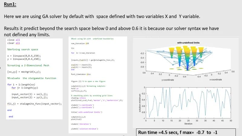
%Run1 using GA with  undefined boundaries

num_iteration =50

tic

for  k= 1:num_iteration


[inputs,fval(k)] = ga(@stalagmite_func,2);

xval(k) = inputs(1);
yval(k) = inputs(2);
end

Run1_timetaken =toc


figure (1) % to open a new figure 

subplot(2,1,1) %creating subplots
hold on
surfc(xx,yy,f);

% smoothing plots by avoiding grid lines
shading interp
plot3(xval,yval,fval,'marker','o','markersize',5);

xlabel('x-coordinate')
ylabel('y-coordinate')

title('with-undefined limits')

subplot(2,1,2)
plot(fval)

xlabel('iteration')

ylabel('solution-minimum')


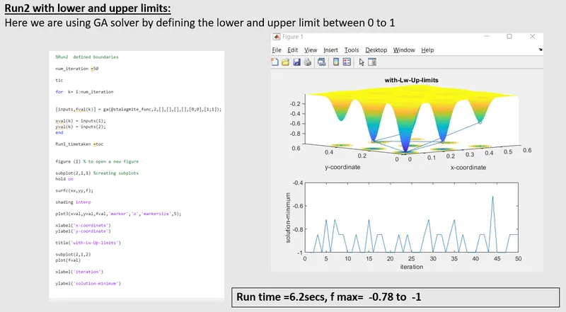
%Run2  defined boundaries

num_iteration =50

tic

for  k= 1:num_iteration


[inputs,fval(k)] = ga(@stalagmite_func,2,[],[],[],[],[0;0],[1;1]);

xval(k) = inputs(1);
yval(k) = inputs(2);
end

Run2_timetaken =toc


figure (2) % to open a new figure 

subplot(2,1,1) %creating subplots
hold on

surfc(xx,yy,f);

shading interp

plot3(xval,yval,fval,'marker','o','markersize',5);

xlabel('x-coordinate')
ylabel('y-coordinate')

title('with-Lw-Up-limits')

subplot(2,1,2)
plot(fval)

xlabel('iteration')

ylabel('solution-minimum')

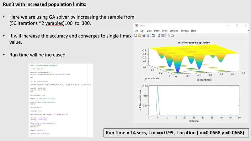
%Run3  increased sample /population

num_iteration =50

options = optimoptions('ga')
options = optimoptions(options,"PopulationSize",300)

tic

for  k= 1:num_iteration

[inputs,fval(k)] = ga(@stalagmite_func,2,[],[],[],[],[0;0],[1;1],[],[],options);

xval(k) = inputs(1);
yval(k) = inputs(2);
end

Run3_timetaken =toc

figure (1) % to open a new figure 

subplot(2,1,1) %creating subplots
hold on

surfc(xx,yy,f);

shading interp

plot3(xval,yval,fval,'marker','o','markersize',5);

xlabel('x-coordinate')
ylabel('y-coordinate')

title('with-increased-population')
subplot(2,1,2)
plot(fval)

xlabel('iteration')

ylabel('solution-minimum')