Taylor table method and Matlab code

AIM

To deepen understanding about Numerical Discretization and to learn about Taylor’s Table Method.

OBJECTIVES

To derive the 4th order approximations of the second-order derivative using the following schemes.

1. Central difference
2. Skewed right-sided difference
3. Skewed left-sided difference

To prove that the skewed schemes are fourth-order accurate.

To write a program in MATLAB to evaluate the second-order derivative of a given analytical function f(x)=exp(x).cos(x) and compare it with the 3 numerical approximations that have been derived.

THEORY

Taylor Table Method or the Method of Undetermined Coefficients is a convenient way of forming linear combinations of Taylor Series on a term-by-term basis. The data points considered in the numerical stencil are written row-wise and their corresponding Taylor Series terms are written column-wise.

The 2^nd order derivative of a function has been numerically discretized here using the Central difference, Skewed right-sided difference, and Skewed left-sided difference for a 4^th order approximation.

For Symmetric Schemes (Central Difference), the number of data points (n) to be considered, for a qth order of approximation of a pth order derivative, are given by the formula:

n = p + q - 1

For Skewed Schemes (Right-Sided/ Left Sided Difference), the number of data points(n) to be considered, for a qth order of approximation of a pth order derivative, is given by the formula:

n = p + q

• Fourth-order approximation of a 2^nd order derivative using Central Difference Scheme

Hypothesis equation

`(∂^2 f)/(∂x^2 )=a.f(i-2)+b.f(i-1)+c.f(i)+d.f(i+1)+e.f(i+2)`

Numerical stencil

	f(i)	f’(i)	f’’(i)	f”’(i)	fiv(i)	fv(i)	fvi(i)
a.f(i-2)	a	a.(-2Δx)	`(a.(-2∆x)^2)/(2!)`	`(a.(-2∆x)^3)/(3!)`	`(a.(-2∆x)^4)/(4!)`	`(a.(-2∆x)^5)/(5!)`	`(a.(-2∆x)^6)/(6!)`
b.f(i-1)	b	b.(-Δx)	`(b.(-∆x)^2)/(2!)`	`(b.(-∆x)^3)/(3!)`	`(b.(-∆x)^4)/(4!)`	`(b.(-∆x)^5)/(5!)`	`(b.(-∆x)^6)/(6!)`
c.f(i)	c
d.f(i+1)	d	d.(Δx)	`(d.(∆x)^2)/(2!)`	`(d.(∆x)^3)/(3!)`	`(d.(∆x)^4)/(4!)`	`(d.(∆x)^5)/(5!)`	`(d.(∆x)^6)/(6!)`
e.f(i+2)	e	e.(2Δx)	`(e.(2∆x)^2)/(2!)`	`(e.(2∆x)^3)/(3!)`	`(e.(2∆x)^4)/(4!)`	`(e.(2∆x)^5)/(5!)`	`(e.(2∆x)^6)/(6!)`
`∑("above terms")=(∂^2 f)/(∂x^2 )`	0	0	1	0	0

Only the sum of coefficients of f”(i) is equal to 1 because the derivative which has to be discretized is of second order and hence the sum of coefficients of higher or lower order derivative terms should be zero.

The 5 unknowns in the hypothesis equation (a, b, c, d and e) can be found out using the 5 equations formed with the help of the Taylor series expansion and the Taylor table.

a + b + c + d + e = 0

a.(-2Δx) + b.(-Δx) + c.0 + d.(Δx) + e.(2Δx) = 0

`(a.(-2∆x)^2)/(2!)+ (b.(-∆x)^2)/(2!)+0.c+ (d.(∆x)^2)/(2!)+ (e.(2∆x)^2)/(2!)=1`

`(a.(-2∆x)^3)/(3!)+ (b.(-∆x)^3)/(3!)+0.c+ (d.(∆x)^3)/(3!)+ (e.(2∆x)^3)/(3!)=0`

`(a.(-2∆x)^4)/(4!)+ (b.(-∆x)^4)/(4!)+0.c+ (d.(∆x)^4)/(4!)+ (e.(2∆x)^4)/(4!)=0`

The above equations can be solved for calculating these unknown coefficients in terms of Δx.

Note: To prove that the central difference scheme with the nodes considered here is fourth order accurate, an example has been shown below.

The values of unknown coefficients computed using the matrix inversion technique are given by:

a = -0.0833/(Δx)²

b = 1.3333/(Δx)²

c = -2.5000/(Δx)²

d = 1.3333/(Δx)²

e = -0.0833/(Δx)²

The sum of coefficients of f^v(i):

`(a.(-2∆x)^5)/(5!)+(b.(-∆x)^5)/(5!)+(d.(∆x)^5)/(5!)+(e.(2∆x)^5)/(5!)=(-32a-b+d+32e)((∆x)^5/(5!))=0`

The sum of coefficients of f^vi(i):

`(a.(-2∆x)^6)/(6!)+(b.(-∆x)^6)/(6!)+(d.(∆x)^6)/(6!)+(e.(2∆x)^6)/(6!)=(64a+b+d+64e)((∆x)^6/(6!))≠0`

When the values of a, b, d and e are substituted, the exponent of Δx becomes 4 which implies that the coefficients of f^vi(i) are of fourth order or the expression for the second order derivative is fourth order accurate.

• Fourth order approximation of a 2^nd order derivative using Skewed Right-Sided Difference Scheme

Hypothesis Equation

`(∂^2 f)/(∂x^2 )=a.f(i)+b.f(i+1)+c.f(i+2)+d.f(i+3)+e.f(i+4)+g.f(i+5)`

Numerical stencil

	f(i)	f’(i)	f’’(i)	f”’(i)	fiv(i)	fv(i)	fvi(i)
a.f(i)	a
b.f(i+1)	b	b.(Δx)	`(b.(∆x)^2)/(2!)`	`(b.(∆x)^3)/(3!)`	`(b.(∆x)^4)/(4!)`	`(b.(∆x)^5)/(5!)`	`(b.(∆x)^6)/(6!)`
c.f(i+2)	c	c.(2Δx)	`(c.(2∆x)^2)/(2!)`	`(c.(2∆x)^3)/(3!)`	`(c.(2∆x)^4)/(4!)`	`(c.(2∆x)^5)/(5!)`	`(c.(2∆x)^6)/(6!)`
d.f(i+3)	d	d.(3Δx)	`(d.(3∆x)^2)/(2!)`	`(d.(3∆x)^3)/(3!)`	`(d.(3∆x)^4)/(4!)`	`(d.(3∆x)^5)/(5!)`	`(d.(3∆x)^6)/(6!)`
e.f(i+4)	e	e.(4Δx)	`(e.(4∆x)^2)/(2!)`	`(e.(4∆x)^3)/(3!)`	`(e.(4∆x)^4)/(4!)`	`(e.(4∆x)^5)/(5!)`	`(e.(4∆x)^6)/(6!)`
g.f(i+5)	g	g.(5Δx)	`(g.(5∆x)^2)/(2!)`	`(g.(5∆x)^3)/(3!)`	`(g.(5∆x)^4)/(4!)`	`(g.(5∆x)^5)/(5!)`	`(g.(5∆x)^6)/(6!)`
`∑("above terms")=(∂^2 f)/(∂x^2 )`	0	0	1	0	0	0

Only the sum of coefficients of f”(i) is equal to 1 because the derivative which has to be discretized is of second order and hence the sum of coefficients of higher or lower order derivative terms should be zero.

The 6 unknowns in the hypothesis equation (a, b, c, d, e and g) can be found out using the 6 equations formed with the help of the Taylor series expansion and the Taylor table.

a + b + c + d + e + g = 0

0.a + b.(Δx) + c.(2Δx) + d.(3Δx) + e.(4Δx) + g.(5Δx) = 0

`0.a+ (b.(∆x)^2)/(2!)+(c.(2∆x)^2)/(2!)+ (d.(3∆x)^2)/(2!)+ (e.(4∆x)^2)/(2!)+ (g.(5∆x)^2)/(2!)=1`

`0.a+ (b.(∆x)^3)/(3!)+(c.(2∆x)^3)/(3!)+ (d.(3∆x)^3)/(3!)+ (e.(4∆x)^3)/(3!)+ (g.(5∆x)^3)/(3!)=0`

`0.a+ (b.(∆x)^4)/(4!)+(c.(2∆x)^4)/(4!)+ (d.(3∆x)^4)/(4!)+ (e.(4∆x)^4)/(4!)+ (g.(5∆x)^4)/(4!)=0`

`0.a+ (b.(∆x)^5)/(5!)+(c.(2∆x)^5)/(5!)+ (d.(3∆x)^5)/(5!)+ (e.(4∆x)^5)/(5!)+ (g.(5∆x)^5)/(5!)=0`

The above equations can be solved for calculating these unknown coefficients in terms of Δx.

Note: To prove that the skewed right-sided difference scheme with the nodes considered here is fourth order accurate, an example has been shown below.

The values of unknown coefficients computed using the matrix inversion technique are given by:

a = 3.7500/(Δx)²

b = -12.8333/(Δx)²

c = 17.8333/(Δx)²

d = -13.0000/(Δx)²

e = 5.0833/(Δx)²

g = -0.8333/(Δx)²

The sum of coefficients of f^vi(i):

`(b.(∆x)^6)/(6!)+(c.(2∆x)^6)/(6!)+(d.(3∆x)^6)/(6!)+(e.(4∆x)^6)/(6!)+(g.(5∆x)^6)/(6!)=(b+64c+729d+4096e+15625g)((∆x)^6/(6!))≠0`

When the values of a, b, d and e are substituted, the exponent of Δx becomes 4 which implies that the coefficients of f^vi(i) are of fourth order or the expression for the second order derivative is fourth order accurate.

• Fourth order approximation of a 2^nd order derivative using Skewed Left-Sided Difference Scheme

Hypothesis Equation

`(∂^2 f)/(∂x^2 )=a.f(i)+b.f(i-1)+c.f(i-2)+d.f(i-3)+e.f(i-4)+g.f(i-5)`

Numerical stencil

	f(i)	f’(i)	f’’(i)	f”’(i)	fiv(i)	fv(i)	fvi(i)
a.f(i)	a
b.f(i-1)	b	b.(-Δx)	`(b.(-∆x)^2)/(2!)`	`(b.(-∆x)^3)/(3!)`	`(b.(-∆x)^4)/(4!)`	`(b.(-∆x)^5)/(5!)`	`(b.(-∆x)^6)/(6!)`
c.f(i-2)	c	c.(-2Δx)	`(c.(-2∆x)^2)/(2!)`	`(c.(-2∆x)^3)/(3!)`	`(c.(-2∆x)^4)/(4!)`	`(c.(-2∆x)^5)/(5!)`	`(c.(-2∆x)^6)/(6!)`
d.f(i-3)	d	d.(-3Δx)	`(d.(-3∆x)^2)/(2!)`	`(d.(-3∆x)^3)/(3!)`	`(d.(-3∆x)^4)/(4!)`	`(d.(-3∆x)^5)/(5!)`	`(d.(-3∆x)^6)/(6!)`
e.f(i-4)	e	e.(-4Δx)	`(e.(-4∆x)^2)/(2!)`	`(e.(-4∆x)^3)/(3!)`	`(e.(-4∆x)^4)/(4!)`	`(e.(-4∆x)^5)/(5!)`	`(e.(-4∆x)^6)/(6!)`
g.f(i-5)	g	g.(-5Δx)	`(g.(-5∆x)^2)/(2!)`	`(g.(-5∆x)^3)/(3!)`	`(g.(-5∆x)^4)/(4!)`	`(g.(-5∆x)^5)/(5!)`	`(g.(-5∆x)^6)/(6!)`
`∑("above terms")=(∂^2 f)/(∂x^2 )`	0	0	1	0	0	0

Only the sum of coefficients of f”(i) is equal to 1 because the derivative which has to be discretized is of second order and hence the sum of coefficients of higher or lower order derivative terms should be zero.

The 6 unknowns in the hypothesis equation (a, b, c, d, e and g) can be found out using the 6 equations formed with the help of the Taylor series expansion and the Taylor table.

a + b + c + d + e + g = 0

0.a + b.(-Δx) + c.(-2Δx) + d.(-3Δx) + e.(-4Δx) + g.(-5Δx) = 0

`0.a+ (b.(-∆x)^2)/(2!)+(c.(-2∆x)^2)/(2!)+ (d.(-3∆x)^2)/(2!)+ (e.(-4∆x)^2)/(2!)+ (g.(-5∆x)^2)/(2!)=1`

`0.a+ (b.(-∆x)^3)/(3!)+(c.(-2∆x)^3)/(3!)+ (d.(-3∆x)^3)/(3!)+ (e.(-4∆x)^3)/(3!)+ (g.(-5∆x)^3)/(3!)=0`

`0.a+ (b.(-∆x)^4)/(4!)+(c.(-2∆x)^4)/(4!)+ (d.(-3∆x)^4)/(4!)+ (e.(-4∆x)^4)/(4!)+ (g.(-5∆x)^4)/(4!)=0`

`0.a+ (b.(-∆x)^5)/(5!)+(c.(-2∆x)^5)/(5!)+ (d.(-3∆x)^5)/(5!)+ (e.(-4∆x)^5)/(5!)+ (g.(-5∆x)^5)/(5!)=0`

The above equations can be solved for calculating these unknown coefficients in terms of Δx.

Note: To prove that the skewed left-sided difference scheme with the nodes considered here is fourth order accurate, an example has been shown below.

The values of unknown coefficients computed using the matrix inversion technique are given by:

a = 3.7500/(Δx)²

b = -12.8333/(Δx)²

c = 17.8333/(Δx)²

d = -13.0000/(Δx)²

e = 5.0833/(Δx)²

g = -0.8333/(Δx)²

The sum of coefficients of f^vi(i):

`(b.(-∆x)^6)/(6!)+(c.(-2∆x)^6)/(6!)+(d.(-3∆x)^6)/(6!)+(e.(-4∆x)^6)/(6!)+(g.(-5∆x)^6)/(6!)=(b+64c+729d+4096e+15625g)((∆x)^6/(6!))≠0`

When the values of a, b, d and e are substituted, the exponent of Δx becomes 4 which implies that the coefficients of f^vi(i) are of fourth order or the expression for the second order derivative is fourth order accurate.

MATLAB CODE

The code for the given function f(x)=exp(x).cos(x)

function y = f_tt(x)

  y = (exp(x))*cos(x);

end

The code for finding the Taylor Table Coefficients for given order of derivative, order of approximation and discretization scheme.

%   TAYLOR'S TABLE
function [A,C,B] = taylor_table(od,oa,scheme_type)

    if (scheme_type == 'skew_righsided_diff')
    
    %   Hypothesis equation
    %   f^od(i) = a*f(i) + b*f(i+1) + c*f(i+2) + d*f(i+3) + ...(od+oa) terms

        C = zeros(od+oa,1);
        C(od+1) = 1;
        
        for j=1:od+oa
            for i=1:od+oa
                A(i,j) = ((j-1)^(i-1))/factorial(i-1);
            end
        end
       
    elseif (scheme_type == 'skew_leftsided_diff')
    
    %   Hypothesis equation
    %   f^od(i) = a*f(i) + b*f(i-1) + c*f(i-2) + d*f(i-3) + ...(od+oa) terms
    
        C = zeros(od+oa,1);
        C(od+1,1) = 1;
        
        for j=1:od+oa
            for i=1:od+oa
                A(i,j) = ((1-j)^(i-1))/factorial(i-1);
            end
        end
      
    elseif (scheme_type == 'symm__central__diff')
    
    %   Hypothesis equation
    %   Either f^od(i) = a*f(i-2) + b*f(i-1) + c*f(i) + d*f(i+1) + ...(od+oa-1) terms
    %   Or f^od(i) = a*f(i-5) + b*f(i-3) + c*f(i-1) + d*f(i+1) + ...(od+oa-1) terms
        
        C = zeros(od+oa-1,1);
        C(od+1,1) = 1;
        if rem(od,2)==0
            for j=1:(od+oa-1)
             for i=1:(od+oa-1)
                    A(i,j) = ((j-(od+oa)/2)^(i-1)/factorial(i-1));
             end
            end
        elseif rem(od,2)==1
            for j=1:(od+oa-1)
             for i=1:(od+oa-1)
                    A(i,j) = ((2*j-(od+oa))^(i-1)/factorial(i-1));
             end
            end
        end
    end
    
    %   A*B = C
    B = (A^(-1))*C;
        
end

Code for main function

% Main function
close all
clear all
clc

%   Different schemes for 4th order approximation of Second order derivative

%   Skewed Right Sided Difference Scheme (Fourth Order)
%   f''(x) = a*f(i) + b*f(i+1) + c*f(i+2) + d*f(i+3) + e*f(i+4) + g*f(i+5)

%   Skewed Left Sided Difference Scheme (Fourth Order)
%   f''(x) = a*f(i) + b*f(i-1) + c*f(i-2) + d*f(i-3) + e*f(i-4) + g*f(i-5)

%   Symmetric Central Difference Scheme (Second Order)
%   f''(x) = a*f(i-2) + b*f(i-1) + c*f(i) + d*f(i+1) + e*f(i+2)

%   Analytical Calculation of f''(x)
%   f''(x)=-2*(exp(x))*sin(x)


% The function taylor_table has been coded to compute the values of the variables in the equations formed using the Taylor Table. 
% Matrix A depicts the coefficients of the variables a,b,c,etc. which are in the LHS of the equations.
% Matrix C depicts the RHS constants of those equations.
% When solved, Matrix B represents the values of these variables a,b,c etc.
% These variables are the coefficients of the terms in Hypothesis Equation.

% % Steps to use the taylor_table function

% Inputs
    % There are only 3 inputs needed: Order of derivative, Order of approximation, Approximation Scheme. 
    % The Approximation Scheme can be "skew_righsided_difference" for Skewed Right Sided Difference Scheme.
    % The Approximation Scheme can be "skew_leftsided_difference" for Skewed Left Sided Difference Scheme.
    % The Approximation Scheme can be "symm__central__difference" for Symmetric Central Difference Scheme.

% Outputs
    % The code gives matrices A, C and B as outputs.

od = 2;
oa = 4;
[A0,C0,B0] = taylor_table(od,oa,'symm__central__diff');
[A1,C1,B1] = taylor_table(od,oa,'skew_leftsided_diff');
[A2,C2,B2] = taylor_table(od,oa,'skew_righsided_diff');

x = pi/3;
dx = linspace(pi/3000,pi/3,100);

%   Analytical Calculation of f''(x)
AC_2nd_order_deriv=(-2)*(exp(x))*sin(x);

for n = 1:length(dx)
     
  %  Skewed Right Sided Difference Scheme (Fourth Order)
  SRSDS_2nd_order_deriv(n) = (B2(1)*f_tt(x) + B2(2)*f_tt(x+dx(n)) + B2(3)*f_tt(x+2*dx(n)) + B2(4)*f_tt(x+3*dx(n)) + B2(5)*f_tt(x+4*dx(n)) + B2(6)*f_tt(x+5*dx(n)))/(dx(n)^2);
  error_SRSDS(n) = abs(SRSDS_2nd_order_deriv(n)-AC_2nd_order_deriv);
  
  %  Skewed Left Sided Difference Scheme (Fourth Order)
  SLSDS_2nd_order_deriv(n) = (B1(1)*f_tt(x) + B1(2)*f_tt(x-dx(n)) + B1(3)*f_tt(x-2*dx(n)) + B1(4)*f_tt(x-3*dx(n)) + B1(5)*f_tt(x-4*dx(n)) + B1(6)*f_tt(x-5*dx(n)))/(dx(n)^2);
  error_SLSDS(n) = abs(SLSDS_2nd_order_deriv(n)-AC_2nd_order_deriv);
  
  %  Symmetric Central Difference Scheme (Second Order)
  SCDS_2nd_order_deriv(n) = (B0(1)*f_tt(x-2*dx(n)) + B0(2)*f_tt(x-1*dx(n)) + B0(3)*f_tt(x) + B0(4)*f_tt(x+dx(n)) + B0(5)*f_tt(x+2*dx(n)))/(dx(n)^2);
  error_SCDS(n) = abs(SCDS_2nd_order_deriv(n)-AC_2nd_order_deriv);
  
end

% Plotting
figure(1)
plot(dx,SCDS_2nd_order_deriv,'-s',dx,SLSDS_2nd_order_deriv,'-p',dx,SRSDS_2nd_order_deriv,'-o',dx,AC_2nd_order_deriv,'-h');
legend('Symmetric Central Difference Scheme','Skewed Left-Sided Difference Scheme','Skewed Right-Sided Difference Scheme','Analytical Calculation');
ylabel('Second Order Derivative');
xlabel('dx');

figure(2)
plot(dx,error_SCDS,'-s',dx,error_SLSDS,'-p',dx,error_SRSDS,'-o');
legend('Symmetric Central Difference Scheme','Skewed Left-Sided Difference Scheme','Skewed Right-Sided Difference Scheme');
ylabel('Absolute error');
xlabel('dx');

figure(3)
loglog(dx,error_SCDS,'-s',dx,error_SLSDS,'-p',dx,error_SRSDS,'-o');
legend('Symmetric Central Difference Scheme','Skewed Left-Sided Difference Scheme','Skewed Right-Sided Difference Scheme');
ylabel('Absolute error');
xlabel('dx');

RESULTS AND DISCUSSIONS

The plot shown below is the calculated values of Second Order Derivative using different approximations vs the grid size (dx).

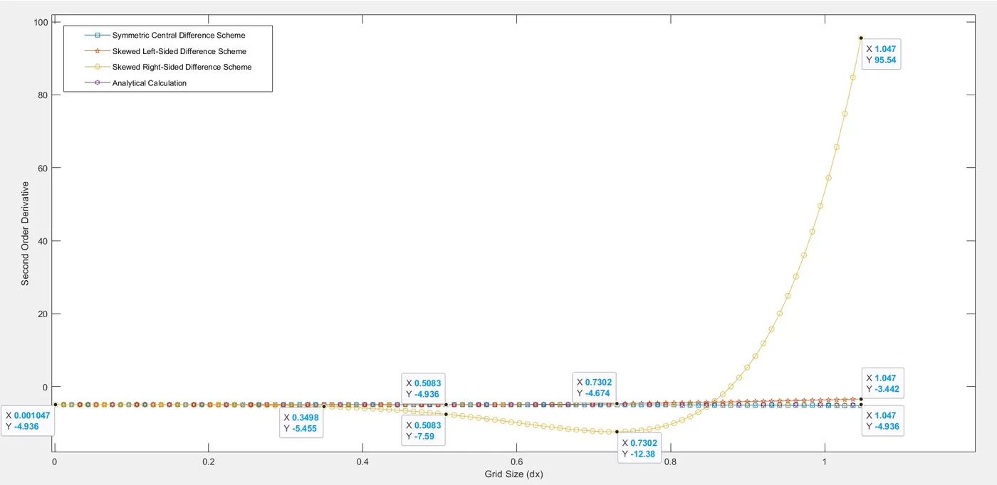
As evident from the plot, the Skewed Right-Sided Difference Scheme seems to diverge greatly as the grid size increases. It should be noted that the analytical value of the second order derivative is -4.9357.

To understand variation of error with respect to the grid size, the following curve has been plotted.

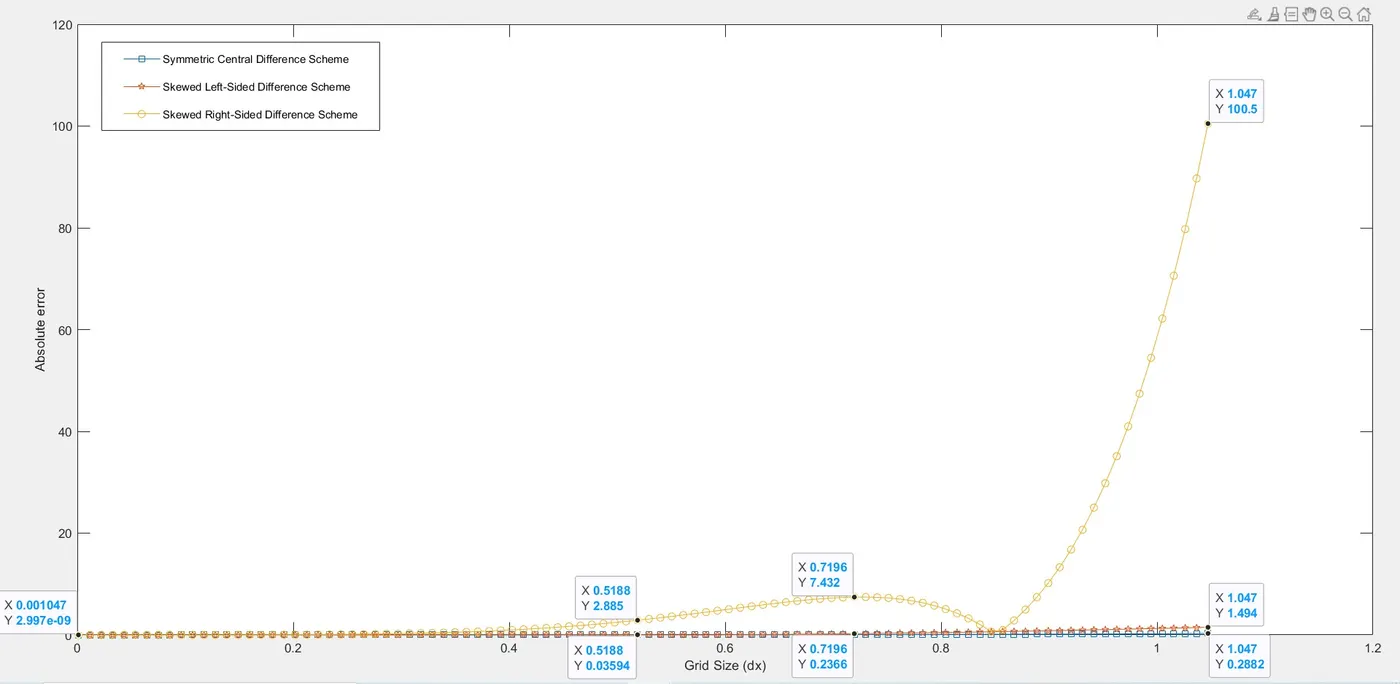
The error term has been calculated as the absolute value of the difference between the approximation and the analytical value. This explains the shape of the curve of the Skewed Right-Sided Difference Scheme. There is a sufficient difference in the order of errors for Central Difference and Skewed Left-Sided Difference Schemes which is not appreciated in the above graph. For this reason, a loglog plot has been plotted below.

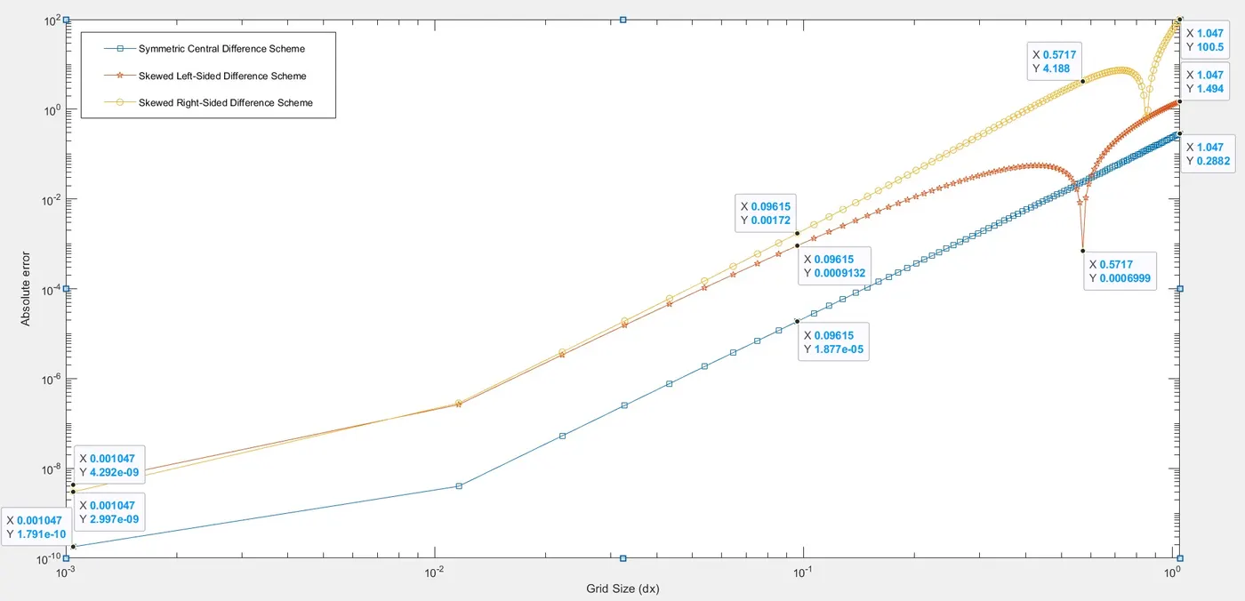
The above plot clearly shows the variations in errors with respect to grid size for all the approximations. The error for Skewed Left-Sided Difference Scheme falls below the Central Difference Scheme for some values of grid size for this particular value of x. For most of the range of dx, the error values are minimum for Central Difference Scheme. The effect of round-off errors can also be seen as the slopes of all the three curves begin to decrease for values of dx below 1e-2.

CONCLUSIONS

• This variation of errors for different approximations is dependent on the function as well as the point at which the function is evaluated.
• The Central Difference Scheme is more accurate (for most values of grid size) and requires lesser number of data points for the same order of approximation.
• The rate of convergence is higher for Central Difference Schemes as compared to the Skewed Schemes.
• However, the Central Difference Schemes cannot be applied at the boundary nodes as they require information from both sides of the node. The Skewed Schemes here have an edge over the Central Difference Schemes as they take information only from one particular side of the node.
• Skewed Schemes tend to gain utmost importance at boundary nodes because Central Difference Scheme fails there.