Numerical discretization for a given function for different ranges of grid size
AIM
To broaden the understanding about numerical discretization and ponder upon the variation of errors in various discretization schemes with the grid size.
OBJECTIVE
To compute the first order derivative of a function `f(x) = (sin (x))/x^3` numerically and analytically.
To find out the first order, second order and fourth order approximations for the first order derivative.
Evaluate the error values and discuss the ways in which they can be visualized in the best way possible.
THEORY
Using the Taylor Series expansions,
`"1st Order Forward Difference Approximation," f^I(x) = (f(x+∆x)-f(x))/(∆x) + o(Δx)`
The truncation error is of the order of Δx, hence the above formulation is first order approximate.
`"1st Order Backward Difference Approximation," f^I(x) = (f(x)-f(x-∆x))/(∆x) + o(Δx)`
The truncation error is of the order of Δx, hence the above formulation is first order approximate.
`"2nd Order Central Difference Approximation," f^I(x) = (f(x+∆x)-f(x-∆x))/(2∆x) + o(Δx)^2`
The truncation error is of the order of (Δx)2, hence the above formulation is second order approximate.
`"4th Order Central Difference Approximation," f^I(x) = (f(x-2∆x)-8f(x-∆x)+8f(x+∆x)-f(x+2∆x))/(12∆x) + o(Δx)^4`
The truncation error is of the order of (Δx)4, hence the above formulation is fourth order approximate.
Analytically, by definition
`f^' (x)=lim_(∆x→0)[(f(x+∆x)-f(x))/(∆x)]`
Now, the function given here is:
`f(x) = (sin (x))/x^3`
Using the product rule,
`(df(x))/dx=f^' (x)=sinx.((-3))/x^4 +cosx/x^3`
This is the analytical expression for the first order derivative.
Error
Error for each difference approximation has been calculated as:
Error = Absolute value of (Numerical Approximation – Actual Value calculated using the analytical expression)
Variation of the error with grid size
Neglecting the absoluteness of the error term for some time and considering `∆x≈dx` , it can be said that,
`"1st Order Forward Difference Approximation Error" = (f(x+dx)-f(x))/dx-f^' (x) = ((sin(x+dx))/(x+dx)^3 -(sin(x))/x^3 )/dx-[sin(x).((-3))/x^4 +(cos(x))/x^3 ]`
`"1st Order Backward Difference Approximation Error" = (f(x)-f(x-dx))/dx-f^' (x) = ((sin(x))/(x)^3 -(sin(x-dx))/(x-dx)^3 )/dx-[sin(x).((-3))/x^4 +(cos(x))/x^3 ]`
`"2nd Order Central Difference Approximation Error" = (f(x+dx)-f(x-dx))/(2dx)-f^' (x) = ((sin(x+dx))/(x+dx)^3 -(sin(x-dx))/(x-dx)^3 )/(2dx)-[sin(x).((-3))/x^4 +(cos(x))/x^3 ]`
`"4th Order Central Difference Approximation Error" = (f(x-2dx)-8f(x-dx)+8f(x+dx)-f(x+2dx))/(12dx) -f^' (x)`
`"4th Order Central Difference Approximation Error" = ((sin(x-2dx))/(x-2dx)^3 -(8sin(x-dx))/(x-dx)^3 +(8sin(x+dx))/(x+dx)^3 -(sin(x+2dx))/(x+2dx)^3 )/(12dx) -[sin(x).((-3))/x^4 +(cos(x))/x^3 ]`
It can be easily said that as the value of dx increases and reaches towards an infinite value, the error term (for each approximation) tends to attain a constant value which is equal to `-f^' (x)`(i.e. the analytical expression of first order derivative with a negative sign), which is a constant for a particular value of x. This has been aptly demonstrated computationally in the results and discussion section of this report. If the value of dx decreases and reaches towards zero, the error terms tend to attain zero value. L-Hospital’s rule was used to calculate the `lim_(dx→0)("error terms")` because of the form encountered`
Note: The discussion above is strictly limited to the given function `f(x) = (sin(x))/x^3`.
Now, all this discussion on error values is based on analytical grounds, when we try to calculate the `lim_(dx→∞)("error terms")` and `lim_(dx→0)("error terms")`.
However, when we try to demonstrate the effect of decrement in grid size computationally, a new error type (the round off error) creeps in. This is because the computation power of the computer is fixed and hence, it tends to round-off the numbers to some significant figure.
Total Numeric Error = Round-off Error + Truncation Error
The results and discussions section provides more insight on this topic.
Variation of the slope of error-grid size plot
The slope of the error vs grid size plot can be mathematically represented as `(d("error term"))/(d(dx))`.
Now, each error term, when differentiated (with respect to dx), the exponent of the dx term in the denominator increases by 1.
For example, considering the backward difference scheme of first order:
`(d("1st order backward difference error"))/(d(dx))= d/(d(dx)) [(f(x)-f(x-dx))/dx-f^' (x)]`
Since, `d/dx [f^' (x)]=0` because `f^'(x)` can be at best a function of x, not dx.
Hence, `d/(d(dx)) [(f(x)-f(x-dx))/dx-f^' (x)]= d/(d(dx)) [(f(x)-f(x-dx))/dx]`
`d/(d(dx)) [(f(x)-f(x-dx))/dx]=[f(x)-f(x-dx)].((-1))/(dx)^2 + 1/dx.(-1).d/dx [f(x-dx)]`
Considering the function provided here:
`d/(d(dx)) [(f(x)-f(x-dx))/dx]=-[(sinx)/x^3 -(sin(x-dx))/(x-dx)^3 ].1/(dx)^2 - [1/dx].d/dx [(sin(x-dx))/(x-dx)^3 ]`
`d/(d(dx)) [(f(x)-f(x-dx))/dx]=-[(sinx)/x^3 -(sin(x-dx))/(x-dx)^3 ].1/(dx)^2 + [1/dx].[(cos(x-dx))/(x-dx)^3 +(sin(x-dx))/(x-dx)^4 ]`
It can be easily said that for the given function,
`lim_(dx→∞)d/(d(dx)) [(f(x)-f(x-dx))/dx-f^' (x)]=0`
So, we can say that, for the given function, the slope of the error vs dx plot becomes zero as dx approaches an infinitely large value.
For this function, it is going to be the same for all the approximations. This is because the exponent of dx in the denominator increases on differentiation without substantial change in the numerator. All the approximations, attain a fairly constant value of error when dx starts to increase beyond a certain number. This has been demonstrated in the results and discussions section.
MATLAB CODE
%   The function f(x)
function y = f(x)

    y = (sin(x))/(x^3);

end
% Main Function
close all
clear all
clc
% Different approximations of First order derivative
% Forward difference approximation (First Order)
% f'(x)=[f(x+dx)-f(x)]/dx
% Backward difference approximation (First Order)
% f'(x)=[f(x)-f(x-dx)]/dx
% Central difference approximation (Second Order)
% f'(x)=[f(x+dx)-f(x-dx)]/2dx
% Central difference approximation (Fourth Order)
% f'(x)=[f(x-2dx)-8f(x-dx)+8f(x+dx)-f(x+2dx)]/12dx
% Analytical Calculation of f'(x)
% f'(x)=-3sin(x)/x^4 + cos(x)/x^3
x=pi/3;
% dx varying from a very low value to a low value
% dx=linspace(pi/2500000,pi/2500,500);
% dx varying from a low value to an intermediate value
dx=linspace(pi/25000,pi/25,500);
% dx varying from an intermediate value to a high value
% dx=linspace(pi/250,pi/0.25,500);
% dx varying from a high value to very high value
% dx=linspace(pi/2.5,pi/0.0025,500);
for i=1:length(dx)
% Forward difference approximation (First Order)
FDA_1(i) = [f(x+dx(i))-f(x)]/dx(i);
% Backward difference approximation (First Order)
BDA_1(i) = [f(x)-f(x-dx(i))]/dx(i);
% Central difference approximation (Second Order)
CDA_2(i) = [f(x+dx(i))-f(x-dx(i))]/(2*dx(i));
% Central difference approximation (Fourth Order)
CDA_4(i) = [f(x-2*dx(i))-8*f(x-dx(i))+8*f(x+dx(i))-f(x+2*dx(i))]/(12*dx(i));
end
% Analytical Calculation of f'(x)
AC = [-3*sin(x)/x^4] + [cos(x)/x^3];
for i=1:length(dx)
% Error in Forward difference approximation (First Order)
error_FDA_1(i) = abs(FDA_1(i)-AC);
% Error in Backward difference approximation (First Order)
error_BDA_1(i) = abs(BDA_1(i)-AC);
% Error in Central difference approximation (Second Order)
error_CDA_2(i) = abs(CDA_2(i)-AC);
% Error in Central difference approximation (Fourth Order)
error_CDA_4(i) = abs(CDA_4(i)-AC);
end
error = [(error_FDA_1)' (error_BDA_1)' (error_CDA_2)' (error_CDA_4)'];
% Bar Graph Subplots
figure(1)
subplot(2,2,1)
bar(dx,error_FDA_1)
xlabel('Grid Size (dx)')
ylabel('Error in Forward Difference Approximation')
title('Absolute Error in Forward Difference Approximation')
subplot(2,2,2)
bar(dx,error_BDA_1)
xlabel('Grid Size (dx)')
ylabel('Error in Backward Difference Approximation')
title('Absolute Error in Backward Difference Approximation')
subplot(2,2,3)
bar(dx,error_CDA_2)
xlabel('Grid Size (dx)')
ylabel('Error in Central Difference Approximation')
title('Absolute Error in Central Difference Approximation of Second Order')
subplot(2,2,4)
bar(dx,error_CDA_4)
xlabel('Grid Size (dx)')
ylabel('Error in Central Difference Approximation')
title('Absolute Error in Central Difference Approximation of Fourth Order')
% Loglog Plot
figure(2)
loglog(dx,error_FDA_1,'-s',dx,error_BDA_1,'-h',dx,error_CDA_2,'-o',dx,error_CDA_4,'-+')
xlabel('Grid Size (dx)')
ylabel('Error Values')
legend('Error in Forward Difference Approximation','Error in Backward Difference Approximation','Error in Central Difference Approximation of Second Order','Error in Central Difference Approximation of Fourth Order')
title('LOGLOG Plot of Errors in different approximations with respect to dx')
% Normal plot
figure(3)
plot(dx,error_FDA_1,'-s',dx,error_BDA_1,'-h',dx,error_CDA_2,'-o',dx,error_CDA_4,'-+')
xlabel('Grid Size (dx)')
ylabel('Error Values')
legend('Error in Forward Difference Approximation','Error in Backward Difference Approximation','Error in Central Difference Approximation of Second Order','Error in Central Difference Approximation of Fourth Order')
title('Normal Plot of Errors in different approximations with respect to dx')
% log(dx) vs log(error)
figure(4)
plot(log10(dx),log10(error_FDA_1),'-s',log10(dx),log10(error_BDA_1),'-h',log10(dx),log10(error_CDA_2),'-o',log10(dx),log10(error_CDA_4),'-+')
legend('Forward Difference Approximation','Backward Difference Approximation','Central Difference Approximation of Second Order','Central Difference Approximation of Fourth Order')
xlabel('log10 dx')
ylabel('log10 error')
title('log error vs log dx')
for i=2:length(dx)
slope_error_FDA_1_log(i)= (log10(error_FDA_1(i))-log10(error_FDA_1(i-1)))/(log10(dx(i))-log10(dx(i-1)));
slope_error_BDA_1_log(i)= (log10(error_BDA_1(i))-log10(error_BDA_1(i-1)))/(log10(dx(i))-log10(dx(i-1)));
slope_error_CDA_2_log(i)= (log10(error_CDA_2(i))-log10(error_CDA_2(i-1)))/(log10(dx(i))-log10(dx(i-1)));
slope_error_CDA_4_log(i)= (log10(error_CDA_4(i))-log10(error_CDA_4(i-1)))/(log10(dx(i))-log10(dx(i-1)));
end
figure(5)
subplot(1,3,1)
plot(dx(2:length(dx)),slope_error_FDA_1_log(2:length(dx)),'-s',dx(2:length(dx)),slope_error_BDA_1_log(2:length(dx)),'-h',dx(2:length(dx)),slope_error_CDA_2_log(2:length(dx)),'-o',dx(2:length(dx)),slope_error_CDA_4_log(2:length(dx)),'-+')
% legend('Slope of Forward Difference Approximation Error','Slope of Backward Difference Approximation Error','Slope of 2nd Order Central Difference Approximation Error','Slope of 4th Order Central Difference Approximation Error')
title('Normal Plot of slopes of Error-Grid Size plots')
xlabel('Grid Size (dx)')
ylabel('Slope Values')
subplot(1,3,2)
plot(dx(2:length(dx)),slope_error_FDA_1_log(2:length(dx)),'-s',dx(2:length(dx)),slope_error_BDA_1_log(2:length(dx)),'-h',dx(2:length(dx)),slope_error_CDA_2_log(2:length(dx)),'-o',dx(2:length(dx)),slope_error_CDA_4_log(2:length(dx)),'-+')
% legend('Slope of Forward Difference Approximation Error','Slope of Backward Difference Approximation Error','Slope of 2nd Order Central Difference Approximation Error','Slope of 4th Order Central Difference Approximation Error')
title('Normal Plot of slopes of Error-Grid Size plots')
xlabel('Grid Size (dx)')
ylabel('Slope Values')
subplot(1,3,3)
plot(dx(2:length(dx)),slope_error_FDA_1_log(2:length(dx)),'-s',dx(2:length(dx)),slope_error_BDA_1_log(2:length(dx)),'-h',dx(2:length(dx)),slope_error_CDA_2_log(2:length(dx)),'-o',dx(2:length(dx)),slope_error_CDA_4_log(2:length(dx)),'-+')
legend('Slope of Forward Difference Approximation Error','Slope of Backward Difference Approximation Error','Slope of 2nd Order Central Difference Approximation Error','Slope of 4th Order Central Difference Approximation Error')
title('Normal Plot of slopes of Error-Grid Size plots')
xlabel('Grid Size (dx)')
ylabel('Slope Values')
for i=2:length(dx)
slope_error_FDA_1(i)= ((error_FDA_1(i))-(error_FDA_1(i-1)))/((dx(i))-(dx(i-1)));
slope_error_BDA_1(i)= ((error_BDA_1(i))-(error_BDA_1(i-1)))/((dx(i))-(dx(i-1)));
slope_error_CDA_2(i)= ((error_CDA_2(i))-(error_CDA_2(i-1)))/((dx(i))-(dx(i-1)));
slope_error_CDA_4(i)= ((error_CDA_4(i))-(error_CDA_4(i-1)))/((dx(i))-(dx(i-1)));
end
figure(6)
subplot(2,2,1)
plot(dx(2:length(dx)),slope_error_FDA_1(2:length(dx)),'-s')
xlabel('Grid Size (dx)')
ylabel('Slope of Error in Forward Difference Approximation')
title('Slope of Absolute Error in Forward Difference Approximation')
subplot(2,2,2)
plot(dx(2:length(dx)),slope_error_BDA_1(2:length(dx)),'-h')
xlabel('Grid Size (dx)')
ylabel('Slope of Error in Backward Difference Approximation')
title('Slope of Absolute Error in Backward Difference Approximation')
subplot(2,2,3)
plot(dx(2:length(dx)),slope_error_CDA_2(2:length(dx)),'-o')
xlabel('Grid Size (dx)')
ylabel('Slope of Error in Central Difference Approximation')
title('Slope of Absolute Error in Central Difference Approximation of Second Order')
subplot(2,2,4)
plot(dx(2:length(dx)),slope_error_CDA_4(2:length(dx)),'-+')
xlabel('Grid Size (dx)')
ylabel('Slope of Error in Central Difference Approximation')
title('Slope of Absolute Error in Central Difference Approximation of Fourth Order')
RESULTS AND DISCUSSIONS
This section of the report has been divided into four parts based on the range of grid sizes.
- CASE I [dx varying from very low to low values]
dx = `[pi/2500000,pi/2500]`
Bar Graphs
The bar graphs for the errors of each approximation scheme are shown below.
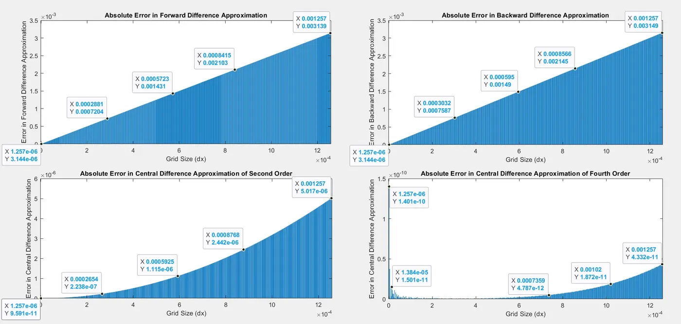
Along with the shapes of the bar graphs, the order of errors on the y-axis should also be noticed.
Normal Plot
Plot of errors in different approximations with respect to dx
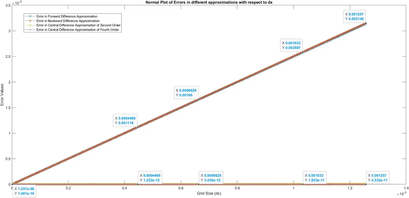
This plot consists of 4 lines (but it appears, that there are only 2); the above 2 seemingly coincident lines in the plot are those for Forward and Backward Difference Approximations and the below 2 seemingly coincident lines in the plot are those for Central Difference of Second Order and Fourth Order respectively. It is quite evident that this plot doesn't show the variation of error values with grid size in a very effective way. This happens because the order of errors for central difference approximations is very much different from the order of errors for forward and backward difference schemes.
NOTE: Due to the incompetency of this plot to demonstrate the variations in error, it will not be considered for remaining cases to save space.
LOGLOG Plot
A LOGLOG plot is the same as a normal plot, except logarithmic scales are used for both the X- and Y- axes. The major axes divisions are equal in length (linear or in arithematic progression) but the values they depict are actually in geometric progression (`10^-4, 10^-6,10^-8` etc.). However, the minor divisions on both the axes are non-linear in length. This kind of plot is extremely useful in plotting data having huge variation in order because the normal plot is unable to capture the variation effectively.
One more peculiarity of LOGLOG plot which was discovered in the process, is that it actually takes the logarithm to the base 10 (i.e. `log_10 a`) for all the data points, plots it on the graph and then takes the antilogarithm of them to display them on the curve. This was discovered when an attempt was made to make a LOGLOG plot of data containing negative values (log of numbers below zero is not defined). This explains minor divisions being non-linear and major divisions being linear. A `log_10("error") vs log_10("dx")`graph has also been plotted below the LOGLOG plot to clarify the minor differences between the two.
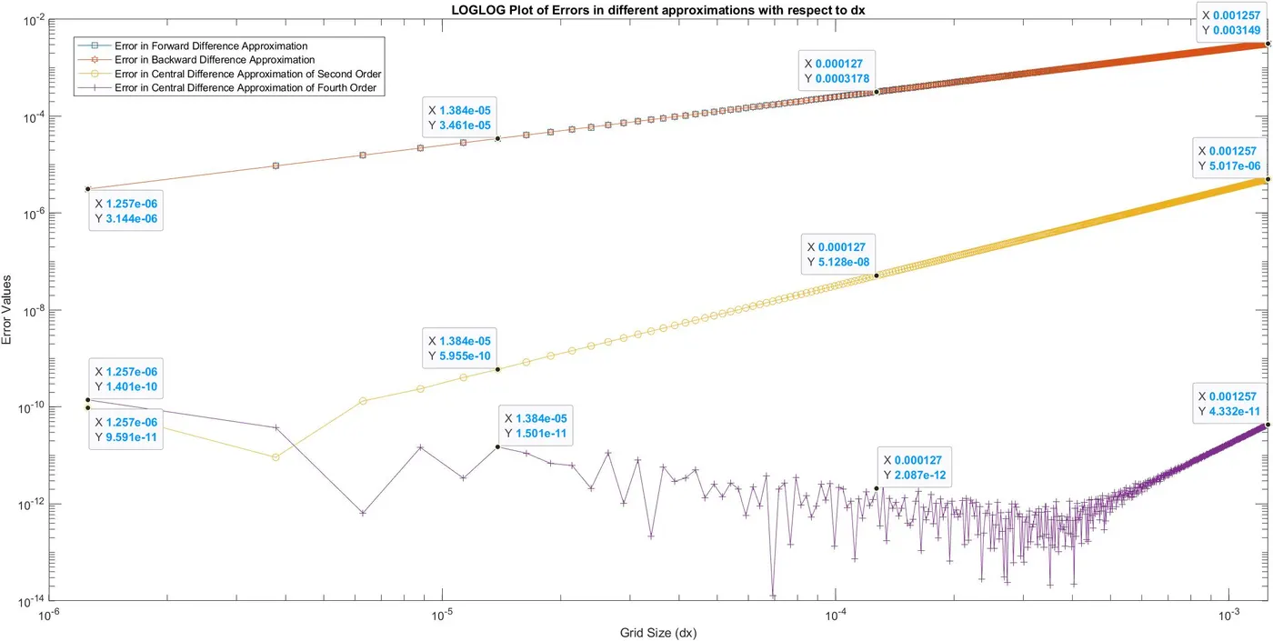
In the curves above, the round-off errors in the extreme left can be noticed, when the errors begin to increase for very low values of grid size in central difference approximations of second and fourth order. For the very low values of grid size considered here, the round-off error for the fourth order scheme increases to such an extent that the total error tends to become more than that of the second order scheme.
Apart from the variation of errors with grid size and the order of errors for different approximations, the X and Y coordinates of the few points denoted, should be noticed. The data points have values which are exactly the same as that in a normal plot.
To support the claims made earlier about the mechanism behind LOGLOG plots, the`log_10("error") vs log_10("dx")` plot below should be looked at.
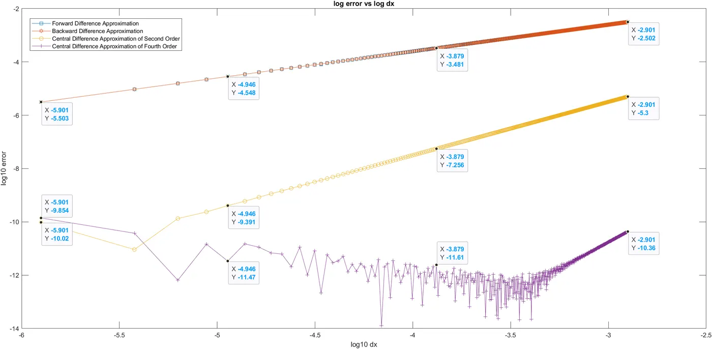
The shapes of the curves in this plot are exactly the same as those in the LOGLOG plot. The X and Y coordinate values are negative which is because the logarithm of any number between 0 and 1 is negative.
Talking about the slopes of these curves, it should be noted that the slopes of first and second order schemes are constant with a variation in slope for the second order scheme for very low dx values. The fourth order scheme shows random fluctuations in the error values. These fluctuations are function specific and of very low order.
However, the slope for the average error (or mean error) in fourth order schemes changes around a dx value of around 1e-3.5, which leads to increament in the error values if the value of dx reduces further. This happens because the round-off error starts playing its role in fourth order schemes quite earlier as compared to the second order schemes. This leads to the total numeric error in fourth order approximation to increase and become more than the total numeric error in second order approximation. The slope of first order approximations remains constant.
An attempt was made to plot the errors in different approximations with respect to dx and following realizations were made:
- A LOGLOG plot is insufficient because the errors may be taken as absolute, but the slopes of the error curves change from positive to negative for low values of grid size (due to rounding off of the numbers) and the LOGLOG plot fails to capture the negative values.
- A Normal plot of the errors is also insufficient, because the errors are of varying orders and hence if plotted together, the variations will not be captured effectively. Plotting separately (as subplots) also doesn't work because the small values of dx tend to magnify the small changes in the error values.
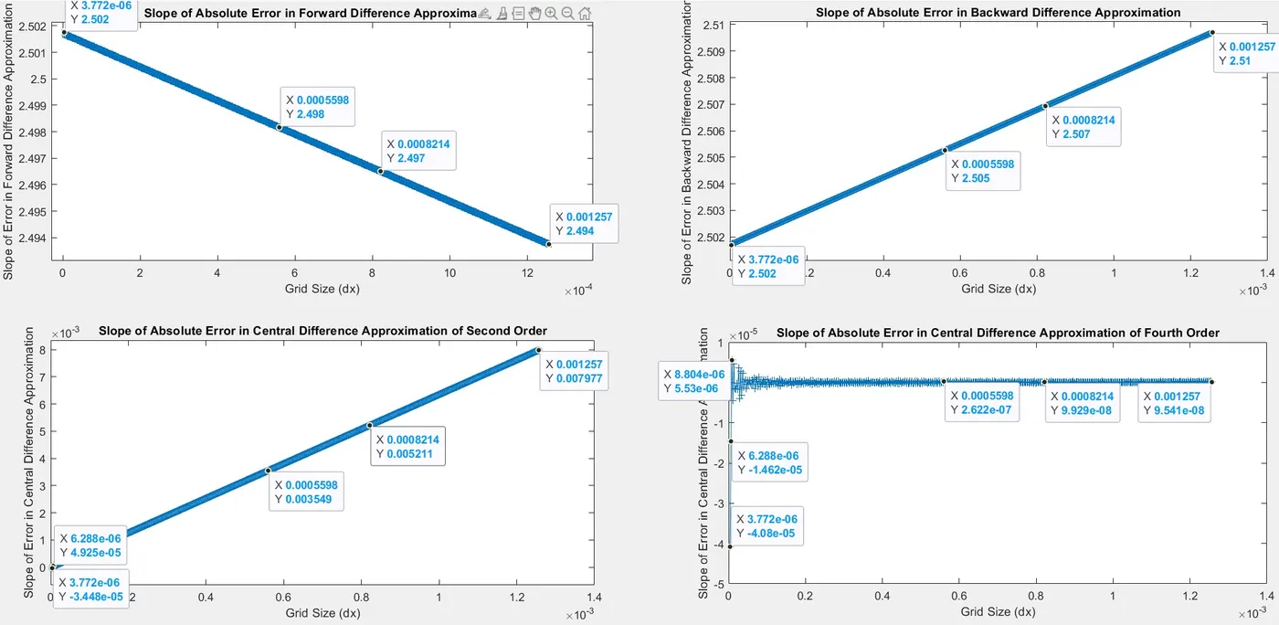
The Y coordinate values are the slopes of error vs dx plots for different approximations. Interestingly, here the Forward and Backward Difference Approximation Errors show decreasing and increasing slope values respectively.
The central difference schemes demonstrate major change of slope for very low values of grid size due to rounding-off of errors, which again is not visualized properly.
- One way to capture the changes in slopes is to make a LOGLOG plot of the slopes of the log error vs log dx plot. It should be noted that the slope values will not be correct here. Since the log error vs log dx graph depicts only the correct trend or pattern of error values, it is expected that correct trend of variation of slopes can be predicted from this plot.
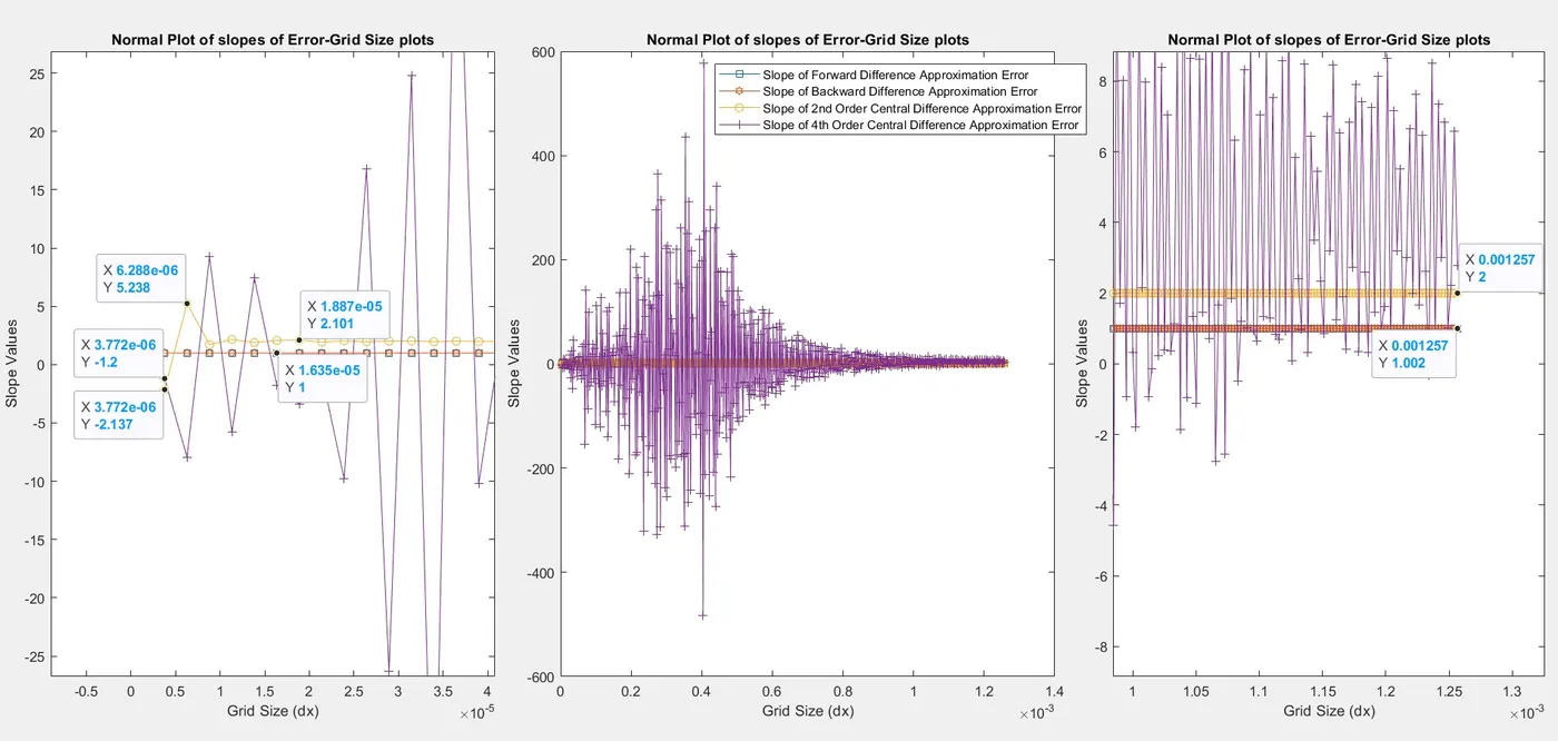
On the left hand side, the left end of the plot has been zoomed in and on the right hand side, the right end of the plot has been zoomed in.
NOTE: The slope values are not the actual slope values of the error vs dx curves but are only indicative of the relative changes in magnitudes. They are the slope values of log error vs log dx curves.
- CASE II [dx varying from low to intermediate values]
dx = `[pi/25000,pi/25]`
Bar Graphs
The bar graphs for the errors of each approximation scheme are shown below.
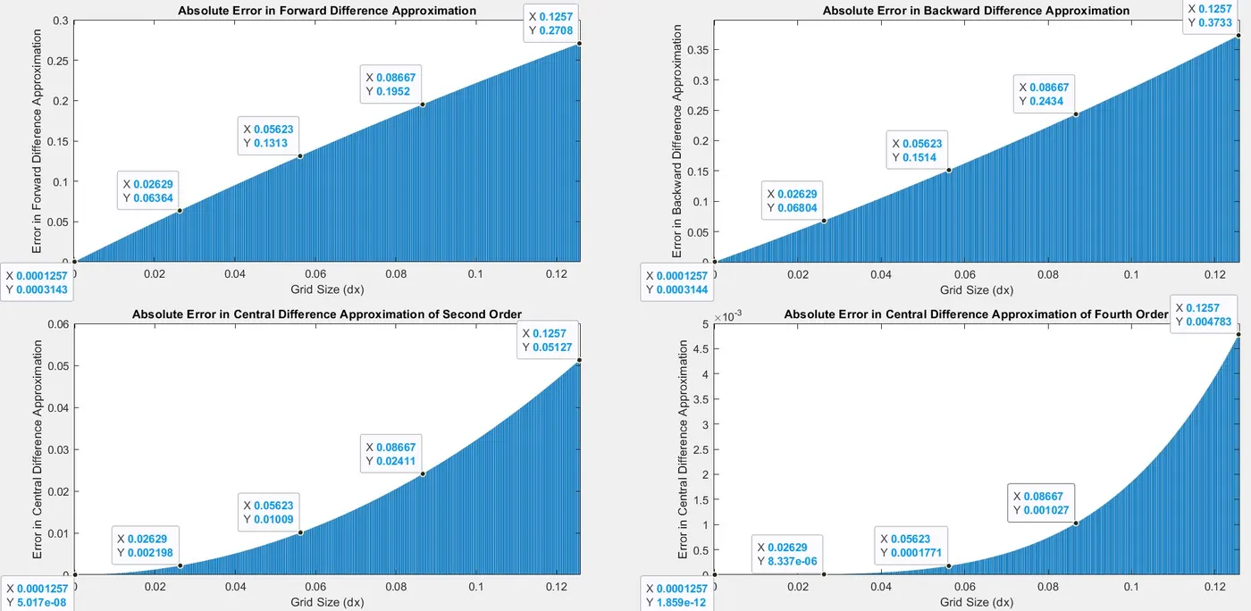
Along with the shapes of the bar graphs, the order of errors on the y-axis should also be noticed.
LOGLOG Plot
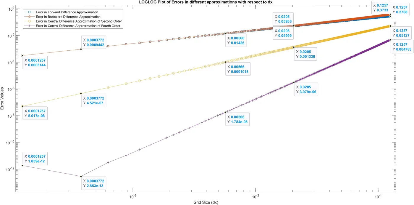
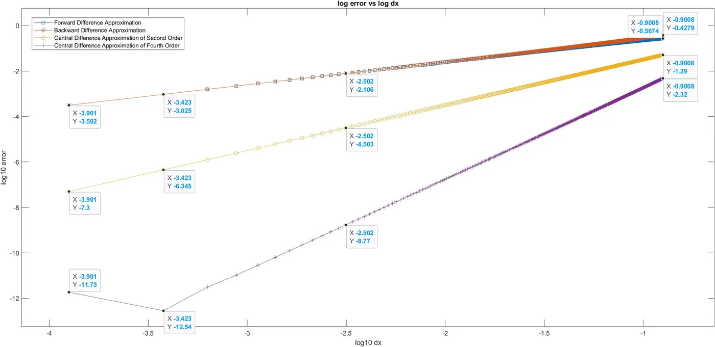
The round-off errors in the extreme left can be noticed, when the errors begin to increase for very low values of grid size in central difference approximation of fourth order. One more interesting behaviour that can be noticed here is that the forward difference approximation curve starts showing visible deviation from the backward difference approximation curve. This happens because the slope of the forward difference scheme is decreasing in nature while that of backward difference scheme is increasing in nature. This difference of slopes can be noticed in the plots below.
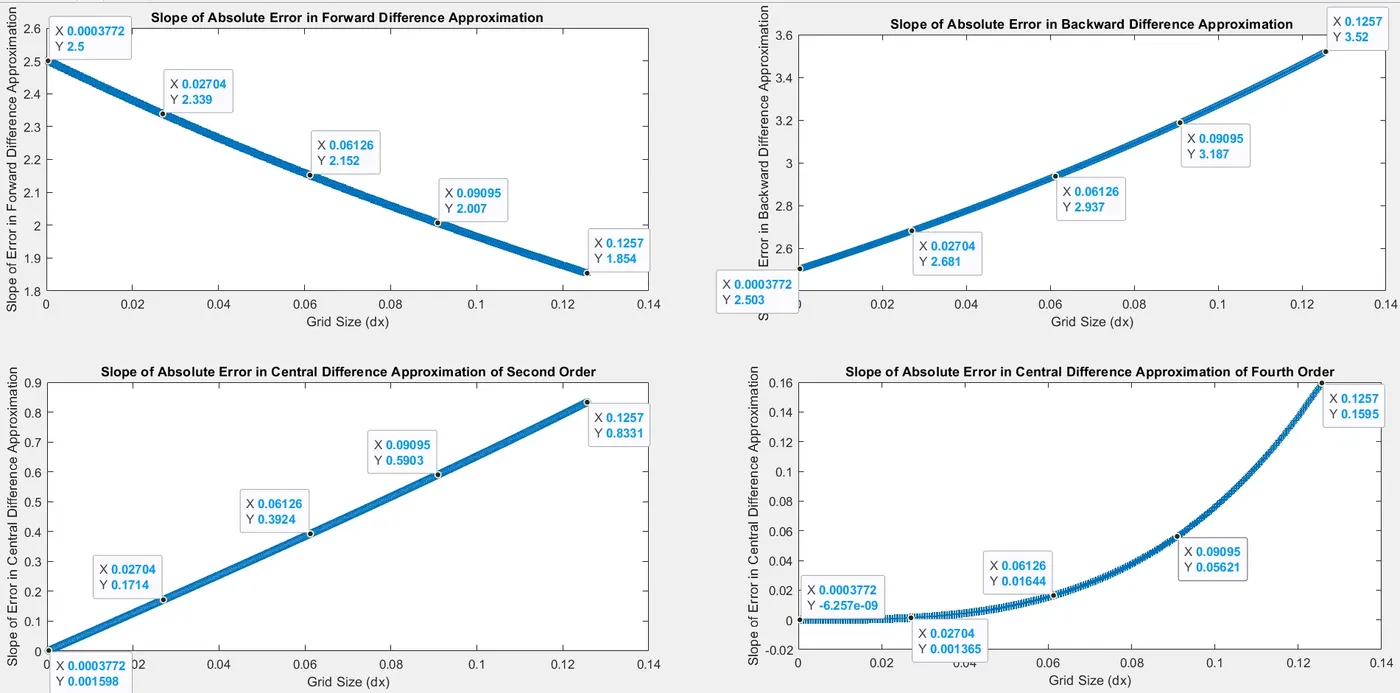
The Y coordinate values are the slopes of error vs dx plots for different approximations. The results of the variation in slopes for first order schemes was visualized in this range for dx in LOGLOG plot. In LOGLOG plot, the small order variations are crunched and the larger order variations are magnified.
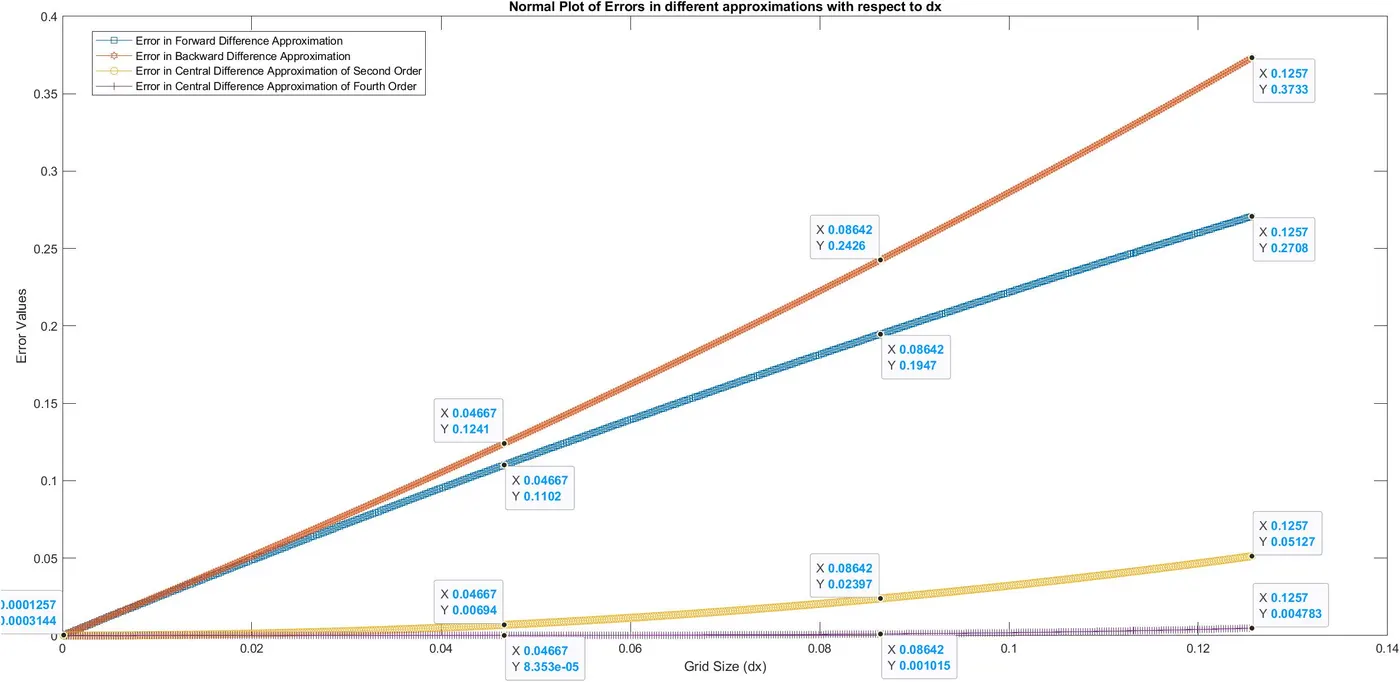
The normal plot for this range of dx maybe interesting to look at (atleast to visualize first order schemes).
The log error vs log dx plot is also shown below and in the plot below that, the slope of this plot is plotted with respect to dx.
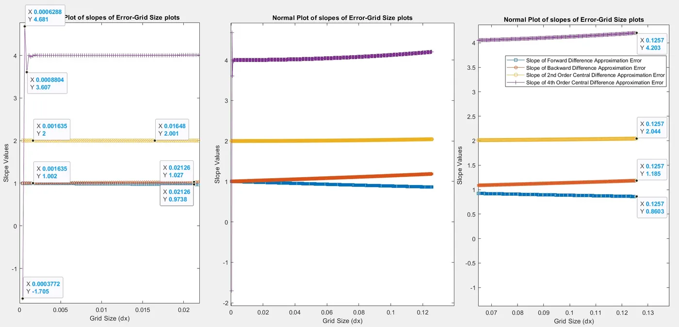
On the left hand side, the left end of the plot has been zoomed in and on the right hand side, the right end of the plot has been zoomed in.
NOTE: The slope values are not the actual slope values of the error vs dx curves but are only indicative of the relative changes in magnitudes. They are the slope values of log error vs log dx curves.
- CASE III [dx varying from intermediate to high values]
dx = `[pi/250,pi/0.25]`
Bar Graphs
The bar graphs for the errors of each approximation scheme are shown below.
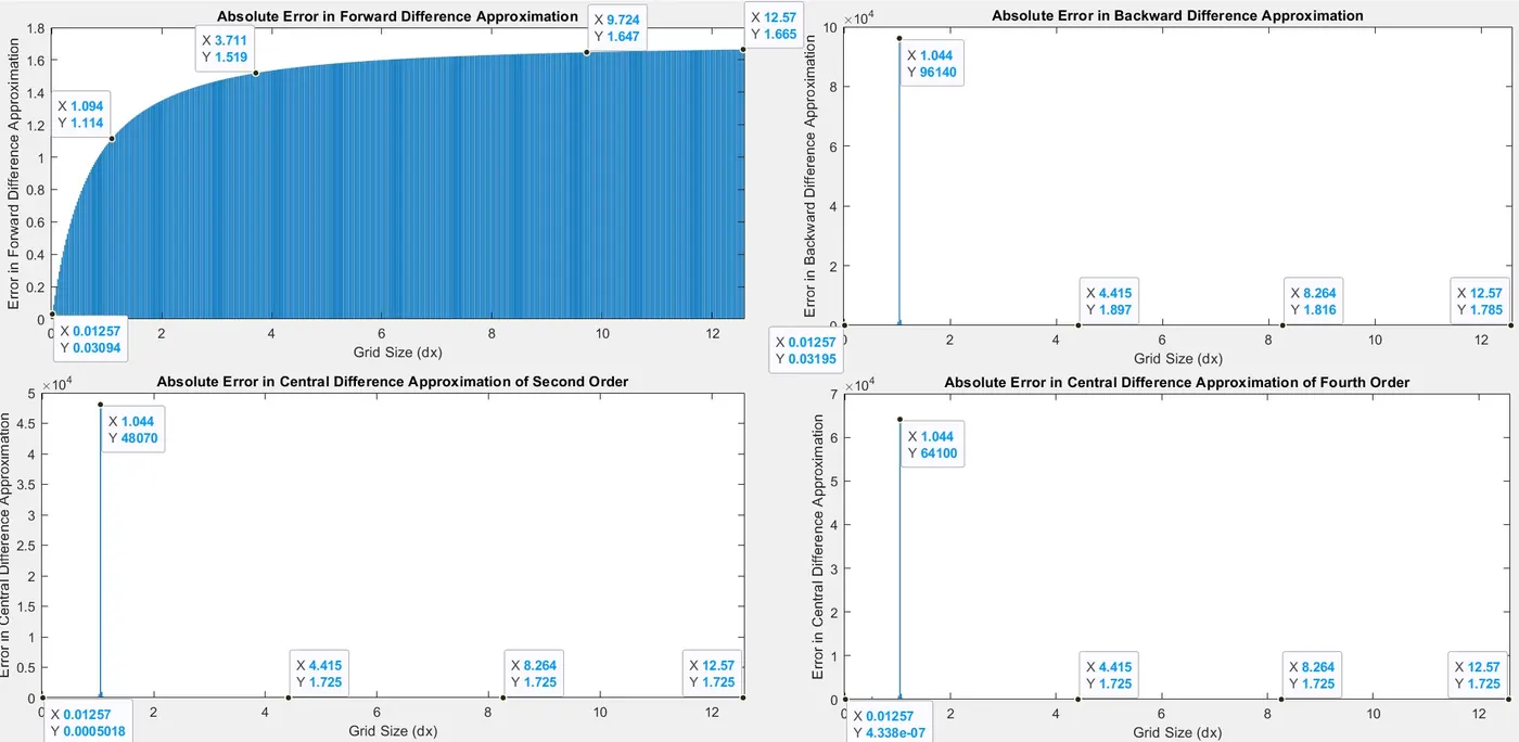
Except the Forward Difference scheme, the bar graphs for the other 3 schemes look very similar in shape. However, if attention is paid to the X and Y coordinate of the spike, it becomes clear that each one of the three schemes, have an error of order 1e4 on just one value of grid size (dx). This vast variation in order of errors is the reason why the bar graph looks like above for the 3 schemes. For the Forward Difference scheme, no such issue is observed.
LOGLOG Plot
Due to this huge variation in order of errors, the normal plot is not a good idea in this case. A LOGLOG plot is shown below to visualize the errors.
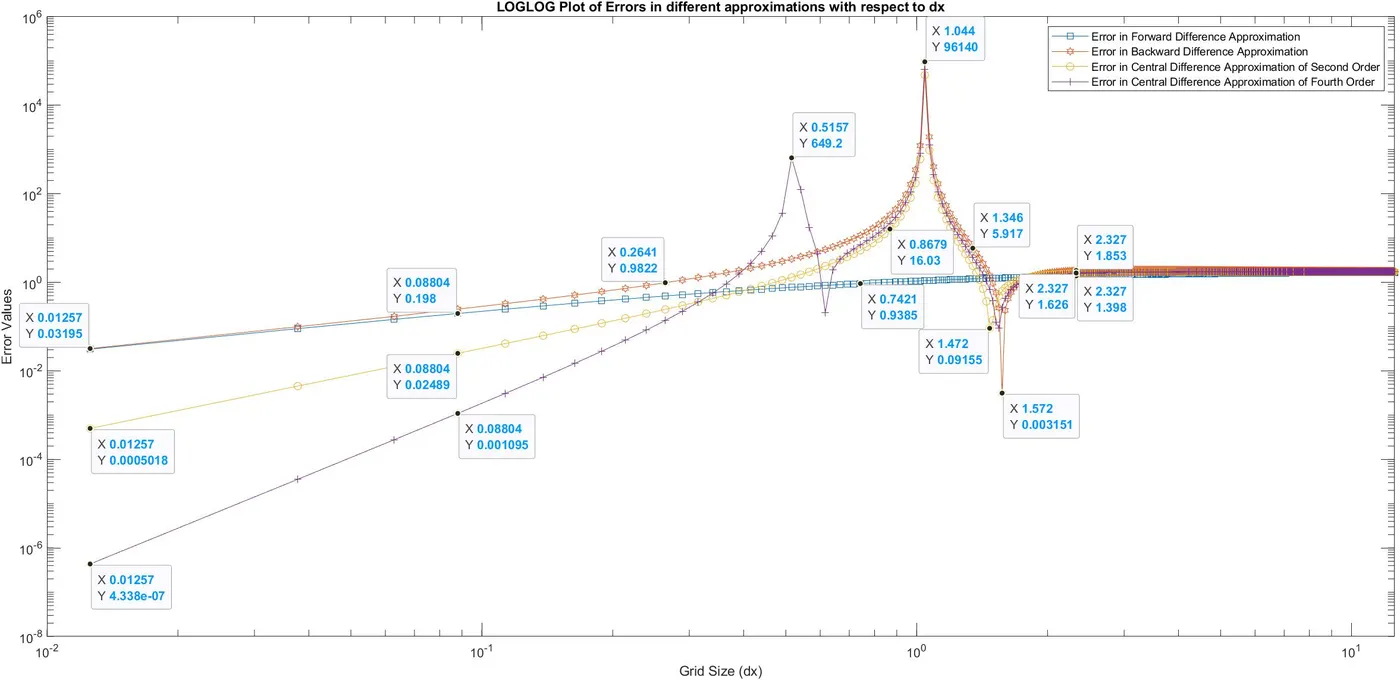
The fourth order approximation shows the maximum fluctuation in errors for this range of grid size, while the forward difference scheme shows none.
The slope of the forward difference shows continuous decreament to reach close to zero as the grid size increases. But the slopes of the remaining 3 difference schemes show fluctuation before their curves seem to flatten out (as proved theoretically also in the theory section above).
The log error vs log dx plot is also shown below and in the plot below that, the slope of this plot is plotted with respect to dx. Since the slopes vary to a great extent, the normal plot is not a good idea.
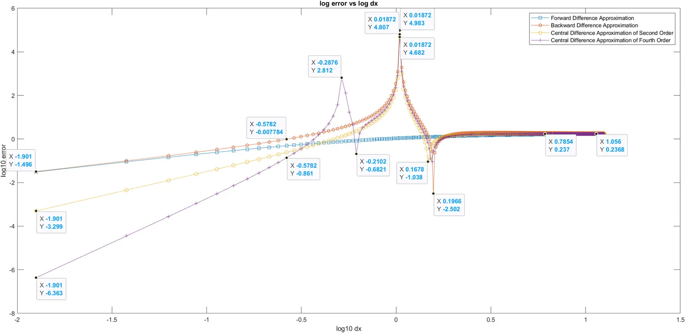
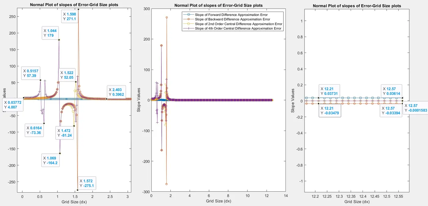
On the left hand side, the left end of the plot has been zoomed in and on the right hand side, the right end of the plot has been zoomed in.
NOTE: The slope values are not the actual slope values of the error vs dx curves but are only indicative of the relative changes in magnitudes. They are the slope values of log error vs log dx curves.
The actual slope variation with grid size has also been shown below to get an idea about the slope values for different approximations.
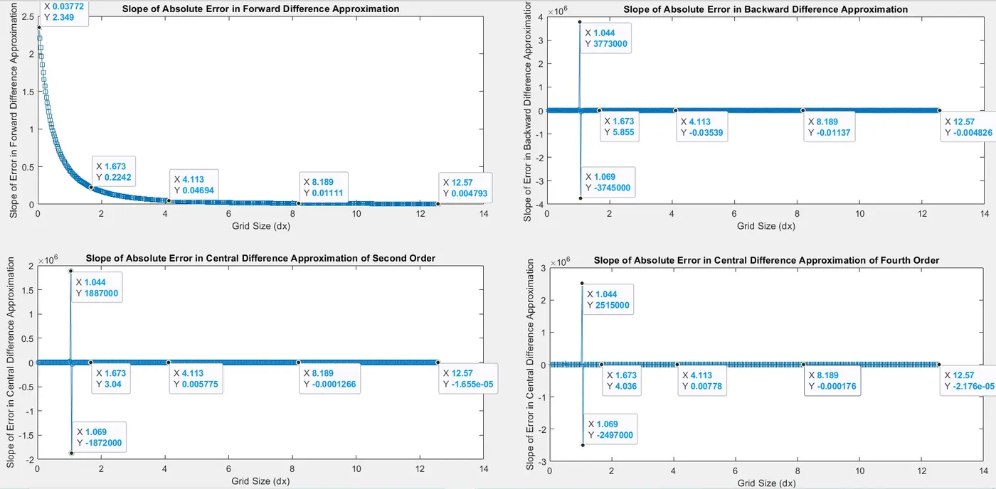
As visible, the slope values towards the larger values of grid size are very close to zero.
- CASE IV [dx varying from high to very high values]
dx = `[pi/2.5,pi/0.0025]`
Bar Graphs
The bar graphs for the errors of each approximation scheme are shown below.
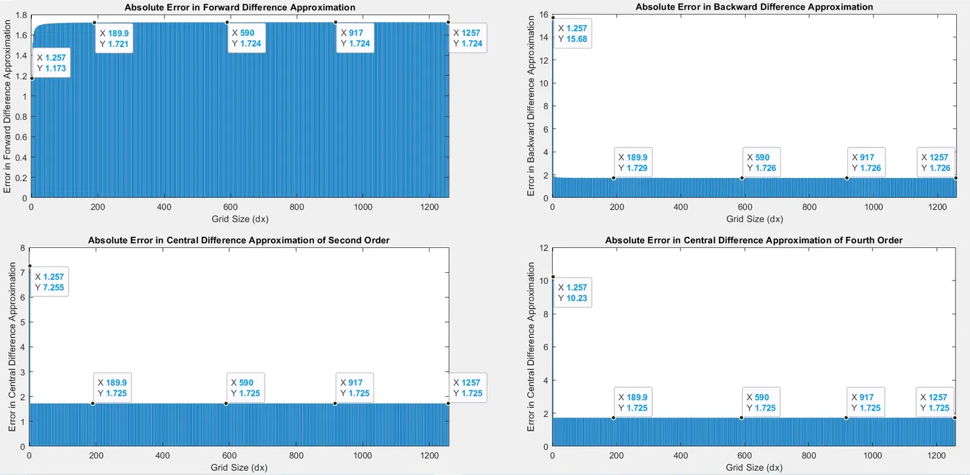
The error values have now become constant and almost of same magnitude. This happens because the denominator in each approximation term is of the form `c(dx)^n`(where n is the order of derivative which is approximated and c is a constant), and now the value of dx has increased to such an extent that the numerator term does not matter much and the overall approximation term tends to zero.
Error = Absolute value of (Numerical Approximation – Actual Value calculated using the analytical expression)
Numerical Approximation ≈ 0
Error = Absolute value of (0 – Actual Value calculated using the analytical expression)
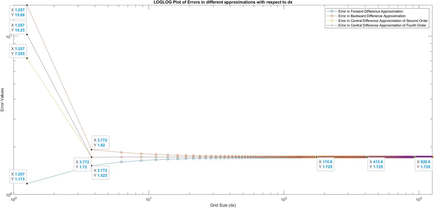
Here the actual value of the first order derivative is -1.7250. It's absolute value will be 1.725 (which is the final error value in the bar graphs for very high dx values).
The slope of the error-dx curves will eventually reach zero value (or very close to zero) as shown below.
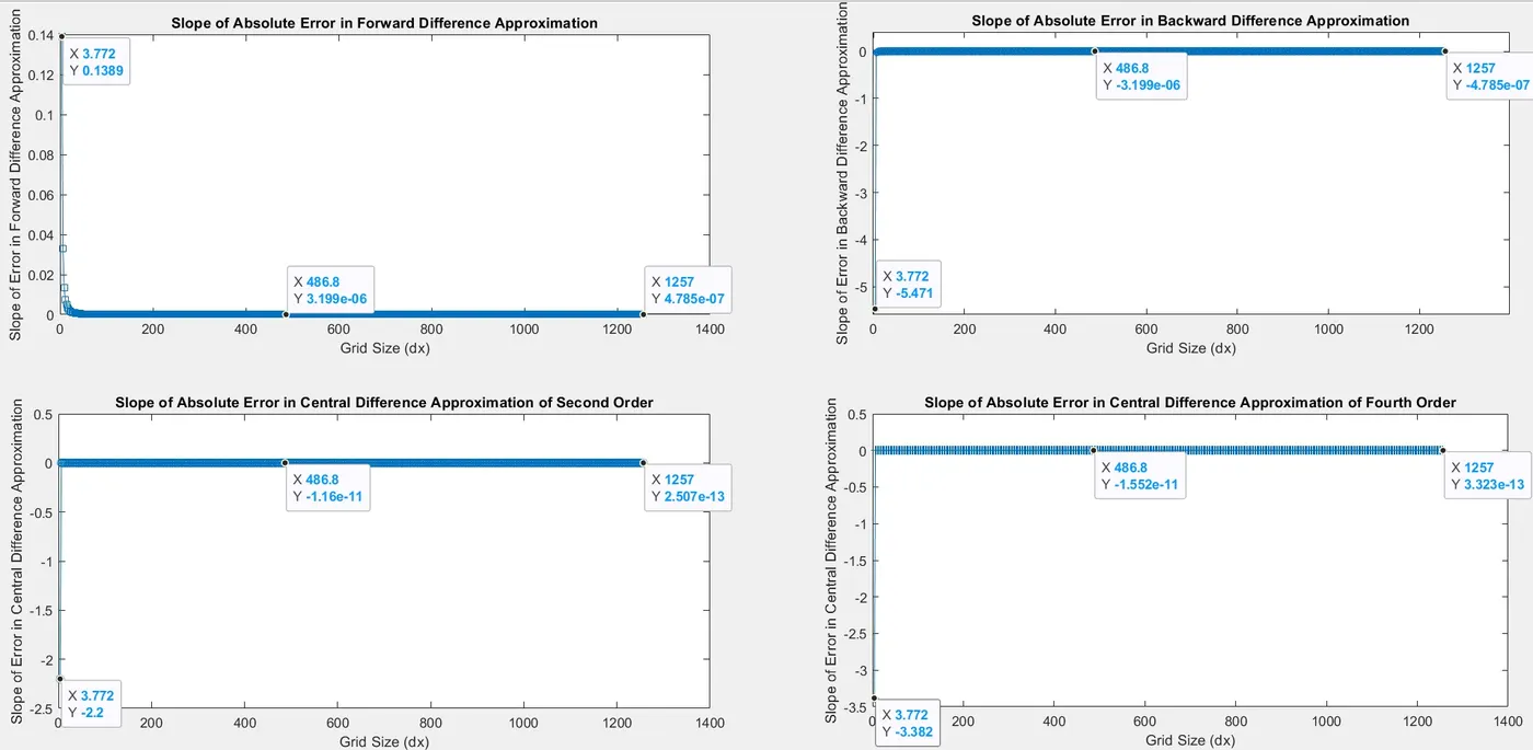
The log error vs log dx plot is not required here as the slopes will behave in the same way in those plots also (very close to zero).
LOGLOG Plot
CONCLUSIONS
- Very low values of grid size are not desirable because of the inclusion of round-off errors in the solution of the system.
- Low to intermediate values of grid size are the most ideal for numerical calculations because of the low truncation error and round-off error.
- High and very high grid sizes don't make much sense and should be avoided for better results.
- As the order of the scheme increases, it becomes more accurate (for appropriate value of grid size) and involves more number of data points.
- Round-off error is not in the control of the user and depends mainly on the system capabilities. With the induction of double-precision, it is not much of a source of worry for analysts.
- Truncation error however, is a function of the grid size and can be reduced by reducing the grid size considered.
- LOGLOG plots are very useful for plotting data that varies a lot in order.