Week 3 - Taylor table method and Matlab code

TAYLOR TABLE METHOD AND MATLAB CODE

Objective : To Derive the following 4th order approximations of the second-order derivative.

1. Central difference

2. Skewed right-sided difference

3. Skewed left-sided difference

Also, prove that your skewed schemes are fourth-order accurate.

INTRODUCTION :

4^th order approximation of second order derivative

1. Central difference scheme:-

To derive for an error of order 4, 2^nd order derivative can be approximated as:-

∂2f∂x2≅f''(x)+Δx^4f^6(x)(CONSTANT)= a⋅f(i−2)+b⋅f(i−1)+c⋅f(i)+d⋅f(i+1)+e⋅f(i+2)

Making the coefficient of second order derivative of x as 1 the equation becomes:-

∂^2/f∂x^2 ≅ f''(x)+Δx^4f^6(x)(CONSTANT)=(a⋅f(i−2)+b⋅f(i−1)+c⋅f(i)+d⋅f(i+1)+e⋅f(i+2))/Δx^2

Thus the coefficient of 2^nd order derivative of x is 1 and while that of other derivatives is 0 and 6^th order derivative is an unknown finite term(which is considered as the error term).

Thus ,in error term the power of delta(x) is 4. This confirms that the approximation is of order 4.

Taylor’s table for the central difference scheme of fourth order approximation of second order derivative:-

	a	-2a	4a/2	-8a/6	16a/24	-32a/120	64a/720
	b	-b	b/2	-b/6	b/24	-b/120	b/720
	c	0	0	0	0	0	0
	d	d	d/2	d/6	d/24	d/120	d/720
	e	2e	4e/2	8e/6	16e/24	32a/120	64e/720
coefficient	0	0	1	0	0	0	-

So now we get some equations,

a+b+c+d+e=0…….(1) ; -2a-b+d+2e=0 ……….(2); 4a+b+d+4e=2 ………(3); -8a-b+d+8e=0 …………(4)

16a+b+d+16e=0 ……….(5).

Solving the equation we get the coefficient of the each term and final equation is as follows:-

a=-1/12; b=4/3; c=-5/2; d=4/3; e=-1/12

∂^2f/∂x^2 ≅ f''(x)+Δx^4f^6(x)(CONSTANT)=(−f(i−2)+16⋅f(i−1)−30⋅f(i)+16⋅f(i+1)−f(i+2)12)Δx^2

2. Skewed right sided difference scheme:-

To derive for an order of 4, 2^nd order derivative can be approximated as :-

∂^2f/∂x^2≅Δx2f''(x)+Δx^6f^6(x)(CONSTANT)=(a⋅f(i)+b⋅f(i+1)+c⋅f(i+2)+d⋅f(i+3)+e⋅f(i+4)+g⋅f(i+5))

Making the coefficient of 2^nd derivative as 1,the equation becomes –

∂^2f/∂x^2≅Δx^2f''(x)+Δx^6f^6(x)(CONSTANT)=(a⋅f(i)+b⋅f(i+1)+c⋅f(i+2)+d⋅f(i+3)+e⋅f(i+4)+g⋅f(i+5))Δx^2

The coefficient of 2^nd derivative is 1 while that of other derivatives 0 and of 6^th derivative of is unknown finite term (which is considered to be the error term).

Thus ,in error term the power of delta(x) is 4. This confirms that the approximation is of order 4.

Taylor’s table for the skewed right sided difference scheme of 4th order approximation of 2^nd order derivative:-

a	0	0	0	0	0	0
	b	b	b/2	b/6	b/24	b/120	b/720
	c	2c	4c/2	8c/6	16c/24	32c/120	64c/720
	d	3d	9d/2	27d/6	81d/24	243d/120	729/720
	e	4e	16e/2	64e/6	256e/24	1024e/120	4096e/720
	g	5g	25g/2	125g/6	625g/24	3125g/120	15625g/720
coefficient	0	0	1	0	0	0

So now we get some equations,

a+b+c+d+e+g=0…….(1); b+2c+3d+4e+5g=0 ……….(2); b+4c+9d+16e+25g=2 ………(3); b+8c+27d+64e+125g=0 …………(4); b+16c+81d+256e+625g=0 ……….(5); b+32c+243d+1024e+3125g…………….(6).

Solving the equation we get the coefficient of the each term and final equation is as follows:-

a=15/4; b=-77/6; c=107/6; d=-13; e=61/12; g=-5/6

∂^2f/∂x^2≅f''(x)+Δx^4f^6(x)(CONSTANT)=(45⋅f(i)−154⋅f(i+1)+214⋅f(i+2)−156⋅f(i+3)+61⋅f(i+4)−10⋅f(i+5))12⋅Δx^2

3. Skewed left sided difference scheme:-

   To derive for an order of 4, 2^nd order derivative can be approximated as :-

   ∂^2f/∂x^2 ≅ Δx^2f′'(x)+Δx^6f^6(x)(CONSTANT)=a⋅f(i)+b⋅f(i−1)+c⋅f(i−2)+d⋅f(i−3)+e⋅f(i−4)+g⋅f(i−5)

   Making the coefficient of 2^nd derivative as 1,the equation becomes –

   ∂^2f/∂x^2≅f''(x)+Δx^4f^6(x)(CONSTANT)=(af(i)+bf(i−1)+cf(i−2)+df(i−3)+ef(i−4)+gf(i−5))/(Δx)^2

   The coefficient of 2^nd derivative is 1 while that of other derivatives 0 and of 6^th derivative of is unknown finite term (which is considered to be the error term).

   Thus ,in error term the power of delta(x) is 4. This confirms that the approximation is of order 4.

   Taylor’s table for the skewed right sided difference scheme of 4th order approximation of 2^nd order derivative:-

	a	0	0	0	0	0	0
	b	-b	b/2	-b/6	b/24	-b/120	b/720
	c	-2c	4c/2	-8c/6	16c/24	-32c/120	64c/720
	d	-3d	9d/2	-27d/6	81d/24	-243d/120	729/720
	e	-4e	16e/2	-64e/6	256e/24	-1024e/120	4096e/720
	g	-5g	25g/2	-125g/6	625g/24	-3125g/120	15625g/720
coefficient	0	0	1	0	0	0	-

So now we get some equations,

a+b+c+d+e+g=0 …….(1);-(b+2c+3d+4e+5g)=0 ……….(2);b+4c+9d+16e+25g=2………(3); -b-8c-27d-64e-125g=0…………(4); b+16c+81d+256e+625g=0……….(5); -b-32c-243d-1024e-3125g…………….(6).

Solving the equation we can get the coefficient of the each term and final equation is as follows:-

a=15/4; b=-77/6; c=107/6; d=-13; e=61/12; g=-5/6

∂^2f/∂x^2 ≅ f''(x)+Δx^4f^6(x)(CONSTANT)=(45⋅f(i)−154⋅f(i+1)+214⋅f(i+2)−156f(i+3)+61f(i+4)−10f(i+5))12⋅〖Δx]^2

Coefficient of above equations were find out using matlab code,so here are the matlab codes to determine the coefficients in different schemes.

MATLAB CODE :

%%solving equations for central difference scheme
clear all
close all 
clc

syms a b c d e 

%equations for central difference scheme
eqn_1= a+b+c+d+e==0;
eqn_2= -2*a-b+d+2*e==0;
eqn_3= 4*a+b+d+4*e==2;
eqn_4= -8*a-b+d+8*e==0; 
eqn_5= 16*a+b+d+16*e==0;

eqn=[eqn_1 eqn_2 eqn_3 eqn_4 eqn_5];

S=solve(eqn)

coef_a= S.a
coef_b= S.b
coef_c= S.c
coef_d= S.d
coef_e= S.e 

%%solving equations for skewed right sided difference scheme


syms a b c d e g

%equations for skewed right sided difference scheme
eqn_1= a+b+c+d+e+g==0;
eqn_2= b+2*c+3*d+4*e+5*g==0;
eqn_3= b+4*c+9*d+16*e+25*g==2;
eqn_4= b+8*c+27*d+64*e+125*g==0; 
eqn_5= b+16*c+81*d+256*e+625*g==0;
eqn_6= b+32*c+243*d+1024*e+3125*g==0;

eqn=[eqn_1 eqn_2 eqn_3 eqn_4 eqn_5 eqn_6];

S=solve(eqn)

coef_a= S.a
coef_b= S.b
coef_c= S.c
coef_d= S.d
coef_e= S.e
coef_g= S.g
%%solving equations for skewed left sided difference scheme


syms a b c d e g

%equations for skewed left sided difference scheme
eqn_1= a+b+c+d+e+g==0;
eqn_2= -(b+2*c+3*d+4*e+5*g)==0;
eqn_3= b+4*c+9*d+16*e+25*g==2;
eqn_4= -b-8*c-27*d-64*e-125*g==0; 
eqn_5= b+16*c+81*d+256*e+625*g==0;
eqn_6= -b-32*c-243*d-1024*e-3125*g==0;

eqn=[eqn_1 eqn_2 eqn_3 eqn_4 eqn_5 eqn_6];

S=solve(eqn);

coef_a= S.a
coef_b= S.b
coef_c= S.c
coef_d= S.d
coef_e= S.e
coef_g= S.g
%programe to compare the errors obtained by different approximation schemes
clear all 
close all 
clc

%analytical function= exp(x)*cos(x)

%analytical derivative=f''(x)= (exp(x))*(cos(x)-sin(x))

x=pi/3;
dx=linspace(pi/4,pi/40000,200);

analytical_derivative= -2*(exp(x))*(sin(x));

for i=1:length(dx)

    [central_diff(i),skewed_right_diff(i),skewed_left_diff(i),central_error(i),skewed_right_error(i),skewed_left_error(i)]=taylor_table_scheme(x,dx(i),analytical_derivative);

end


figure(1)
loglog(dx,central_error,'r')
hold on
loglog(dx,skewed_right_error,'b')
hold on
loglog(dx,skewed_left_error,'g')
xlabel('log(dx)')
ylabel('log(error)')
legend('central difference scheme','skewed right difference scheme','skewed left difference','location','best')
title('comparision of errors for 4th order approximations for a 2nd order derivative using diff. approximation schemes')




figure(2)
plot(dx,central_error,'r')
hold on
plot(dx,skewed_right_error,'b')
hold on
plot(dx,skewed_left_error,'g')
xlabel('dx')
ylabel('error')
legend('central difference scheme','skewed right difference scheme','skewed left difference','location','best')
title('comparision of errors for 4th order approximations for a 2nd order derivative using diff. approximation schemes')

Functions used in this code :

function [central_diff,skewed_right_diff,skewed_left_diff,central_error,skewed_right_error,skewed_left_error]=taylor_table_scheme(x,dx,analytical_derivative)

%numerical derivative
%central difference scheme
central_diff=((-exp_x(x-2.*dx))+(16*exp_x(x-dx))-(30*exp_x(x))+(16*exp_x(x+dx))-(exp_x(x+2.*dx)))./(12*(dx.^2));

%skewed right sided difference scheme
skewed_right_diff=((45*exp_x(x))-(154*exp_x(x+dx))+(214*exp_x(x+2.*dx))-(156*exp_x(x+3.*dx))+(61*exp_x(x+4.*dx))-(10*exp_x(x+5.*dx)))./(12*(dx.^2));

%skewed left sided difference scheme
skewed_left_diff=((45*exp_x(x))-(154*exp_x(x-dx))+(214*exp_x(x-2.*dx))-(156*exp_x(x-3.*dx))+(61*exp_x(x-4.*dx))-(10*exp_x(x-5.*dx)))./(12*(dx.^2));

%errors of numerical discritization
central_error=abs(central_diff-analytical_derivative);
skewed_right_error=abs(skewed_right_diff-analytical_derivative);
skewed_left_error=abs(skewed_left_diff-analytical_derivative);
end

function out = exp_x(x,dx)

out = (exp(x))*(cos(x));

end

OUTPUT :

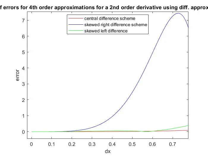
Error approximation curve

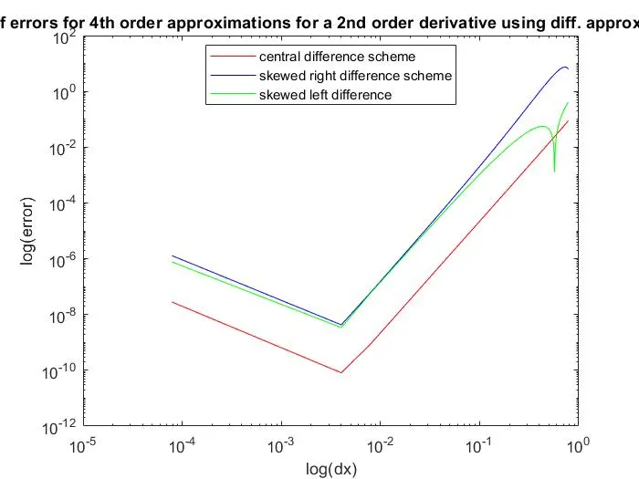
log log curve for error approximation :

CONCLUSION :

1. As seen from the figures the error of the central difference method is very less compared to the skewed methods. also because of its faster convergence rates CDS preffered over skewed methods.

2. Skewed right and left difference methods almost gives the same results in terms of error for a small value of time step.

3. CDS can not be employed at the boundary nodes due to the unavailability of right or eft nodes at the same time. In succh cases the forward and backward differencing schemes are used.