Week 3 - Taylor table method and Matlab code

Aim: Deriving fourth order approximation of second order derivative using Taylor table

Objective:

• Deriving fourth order approximation of second order derivative for central differencing, backward differencing and forward differencing schemes.
• Verify and evaluate these schemes for a given function
• Comparing the numerical approximations with their absolute errors. Determine the usefullness of skewed scheme over central differencing scheme.

Theory:

In mathematics, Taylor series is an infinte sum of terms, that are expressed in terms of the function's derivative at a single point. It can be thus used to approximate values of derivatives at that point using various approximation schemes. This derivative is measured at that point, using the data available around the point. As the name suggests (viz. numerical approximations) certains errors are introduced while evaluating by such methods; the errors are known as truncation errors, which are dependent on powers of spacing. These powers decide the order of the appoximation.

The schemes which we employ are known as finite difference methods. It is a class of numerical techniques using numerical discretization. Three commonly considered schemes are:

1. Forward Difference Scheme / Skewed Right-Side Difference Scheme

`Delta_{h} f(x) = f(x+h) - f(x)`

2. Backward Difference Scheme / Skewed Left-Side Difference Scheme

`Nabla_{h} f(x) = f(x) - f(x-h)`

3. Central Differencing Scheme

`del_{h} f(x) = f(x+h/2) - f(x-h/2)`

In numerical schemes, if the selected nodes are symmetric about the point at which approximation is derived, it is called as central differencing scheme, otherwise it forms a skewed scheme.

Taylor-Table Formulation:

The schemes are formulated as a linear function of node values with constant coefficients. The coefficients are calculated using Taylor table method. Hence if node is chosen as `x`, the approximations can be given as:

Central Difference:

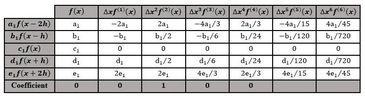
`f''(x) = (a_1f(x-2h) + b_1f(x-h) + c_1f(x) + d_1f(x+h) + e_1f(x+2h))/h^2`

Skewed left-sided difference:

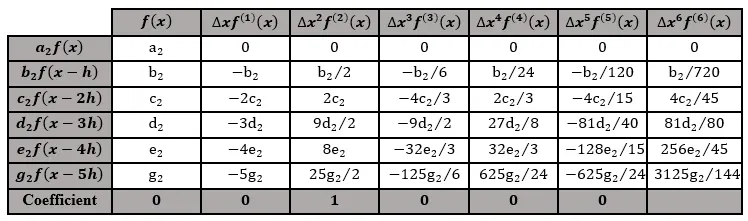
`f''(x) = (a_2f(x) + b_2f(x-h) + c_2f(x-2h) + d_2f(x-3h) + e_2f(x-4h) + g_2f(x-5h))/h^2`

Skewed right-sided difference:

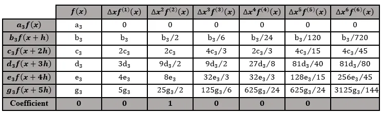
`f''(x) = (a_3f(x) + b_3f(x+h) + c_3f(x+2h) + d_3f(x+3h) + e_3f(x+4h) + g_3f(x+5h))/h^2`

Forward difference scheme:

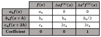
`f''(x) = (a_4f(x) + b_4f(x+h) + c_4f(x+2h))/h^2`

Backward difference scheme:

`f''(x) = (a_5f(x) + b_5f(x-h) + c_5f(x-2h))/h^2`

The taylor table for the above schemes is formed using Taylor series and then comparing the coefficients of each order of the derivatives with LHS. The coefficients are calculated using MATLAB.

Central Difference Scheme:

Skewed Left-Sided Difference Scheme:

Skewed Right-Sided Difference Scheme:

Forward Difference Scheme:

Backward Difference Scheme:

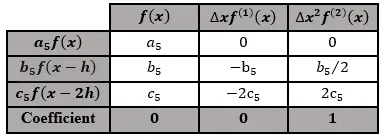
Code:

The code is written in MATLAB.

% A script to evaluate coefficients on Taylor table

clear all
close all
clc

%%% 1: Central difference scheme --> Node(i)=Function(i-2,i-1,i,i+1,i+2)
%%% 2: Skewed left sided difference scheme --> Node(i)=Function(i,i-1,i-2,i-3,i-4,i-5)
%%% 3: Skewed right sided difference scheme --> Node(i)=Function(i,i+1,i+2,i+3,i+4,i+5)
%%% 4: Forward difference scheme (FDS) --> Node(i)=Function(i,i+1,i+2)
%%% 5: Backward difference scheme (BDS) --> Node(i)=Function(i,i-1,i-2)

% Calculating the coefficients for the schemes
% 1. Central
% f"(i) = a1*f(i-2) + b1*f(i-1) + c1*f(i) + d1*f(i+1) + e1*f(i+2)
A1 = [1    1     1  1     1;
     -2   -1     0  1     2;
      2    1/2   0  1/2   2;
     -4/3 -1/6   0  1/6   4/3;
      2/3  1/24  0  1/24  2/3];
B1 = [0 0 1 0 0]';
X1 = A1\B1;
a1 = X1(1);
b1 = X1(2);
c1 = X1(3);
d1 = X1(4);
e1 = X1(5);

% 2. Skewed left sided
% f"(x) = a2*f(i) + b2*f(i-1) + c2*f(i-2) + d2*f(i-3) + e2*f(i-4) + g2*f(i-5)
A2 = [1  1      1     1      1       1;
      0 -1     -2    -3     -4      -5;
      0  1/2    2     9/2    8       25/2;
      0 -1/6   -4/3  -9/2   -32/3   -125/6;
      0  1/24   2/3   27/8   32/3    625/24;
      0 -1/120 -4/15 -81/40 -128/15 -625/24];
B2 = [0 0 1 0 0 0]';
X2 = A2\B2;
a2 = X2(1);
b2 = X2(2);
c2 = X2(3);
d2 = X2(4);
e2 = X2(5);
g2 = X2(6);

% 3. Skewed right sided
% f"(x) = a3*f(i) + b3*f(i+1) + c3*f(i+2) + d3*f(i+3) + e3*f(i+4) + g3*f(i+5)
A3 = [1  1      1     1      1       1;
      0  1      2     3      4       5;
      0  1/2    2     9/2    8       25/2;
      0  1/6    4/3   9/2    32/3    125/6;
      0  1/24   2/3   27/8   32/3    625/24;
      0  1/120  4/15  81/40  128/15  625/24];
B3 = [0 0 1 0 0 0]';
X3 = A3\B3;
a3 = X3(1);
b3 = X3(2);
c3 = X3(3);
d3 = X3(4);
e3 = X3(5);
g3 = X3(6);

% 4. Forward (FDS)
% f"(x) = a4*f(i) + b4*f(i+1) + c4*f(i+2)
A4 = [1  1    1;
      0  1    2;
      0  1/2  2];
B4 = [0 0 1]';
X4 = A4\B4;
a4 = X4(1);
b4 = X4(2);
c4 = X4(3);

% 5. Backward (BDS)
% f"(x) = a5*f(i) + b5*f(i-1) + c5*f(i-2)
A5 = [1   1     1;
      0  -1    -2;
      0   1/2   2];
B5 = [0 0 1]';
X5 = A5\B5;
a5 = X5(1);
b5 = X5(2);
c5 = X5(3);

% Initializing f(x), x and dx
f = @(x) exp(x)*cos(x);
x = pi/3;
dx = linspace(3e-3,5,100);

% Actual second order derivative
d2f = -2*exp(x)*sin(x);

% Initializing error matrix
% err(i,j) --> absolute error for scheme 'i' and dx value of 'j'
err = zeros(5,length(dx));

for i=1:length(dx)
    h = dx(i);
    % Computing approximate derivatives
    d2f1 = (a1*f(x-2*h) + b1*f(x-h) + c1*f(x) + d1*f(x+h) + e1*f(x+2*h))/(h^2);
    d2f2 = (a2*f(x) + b2*f(x-h) + c2*f(x-2*h) + d2*f(x-3*h) + e2*f(x-4*h) + g2*f(x-5*h))/(h^2);
    d2f3 = (a3*f(x) + b3*f(x+h) + c3*f(x+2*h) + d3*f(x+3*h) + e3*f(x+4*h) + g3*f(x+5*h))/(h^2);
    d2f4 = (a4*f(x) + b4*f(x+h) + c4*f(x+2*h))/(h^2);
    d2f5 = (a5*f(x) + b5*f(x-h) + c5*f(x-2*h))/(h^2);
    
    % Computing approximation errors
    err(1,i) = abs(d2f1 - d2f);
    err(2,i) = abs(d2f2 - d2f);
    err(3,i) = abs(d2f3 - d2f);
    err(4,i) = abs(d2f4 - d2f);
    err(5,i) = abs(d2f5 - d2f);
end

% Ploting and comparing the errors in a log-log plot
figure(1)
hold on; grid on;
loglog(dx,err(1,:),'Linewidth',3)
loglog(dx,err(2,:),'Linewidth',3)
loglog(dx,err(3,:),'Linewidth',3)
loglog(dx,err(4,:),'Linewidth',3)
loglog(dx,err(5,:),'Linewidth',3)
xlabel('Log(dx)'); ylabel('Log(error)');
title('Error Comparison for Forward, Backward, Central and Skewed Schemes')
legend('Central','Skewed left-sided','Skewed right-sided','FDS','BDS','location','northwest')
saveas(1,'error_loglogplot.png')

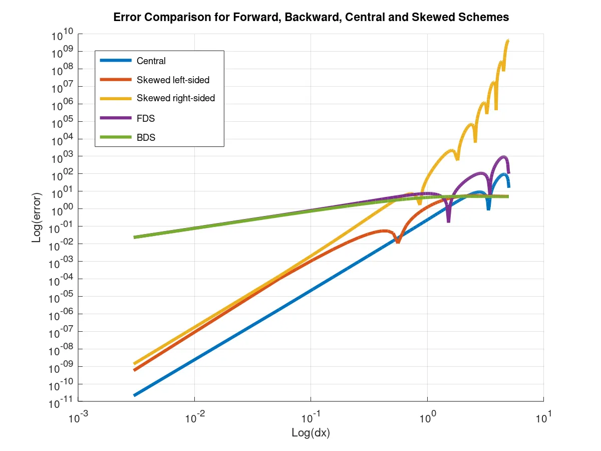
Output:

Results/Conclusion:

• The coefficients for each scheme was deduced.
• From the loglog error plot, we can deduce that the order of error for central differencing scheme is quite lower as compared to the skewed schemes. Moreover, the consistency of central difference scheme is much better than the skewed schemes. (there is no ambiguity in truncation errors in central differencing)
• However, skewed schemes are important in cases where the nodes are closer to the boundaries, thus symmetric arrangement is not possible and/or the solution gets lower accuracy (beacuse of lower order)
• For forward and backward difference schemes, the error seems to get accumulated as the solution proceeds.

References:

• Introducation to CFD using MATLAB and OpenFOAM - Course provided by Skill Lync
• GNU Octave
• Supporting Material: Higher Engineering Mathematics - BS Grewal
• Supporting Material: Mathworks Help Centre
• Supporting Material: Article on Finite Difference