Week 3 - Taylor table method and Matlab code

Derivation of 4th order approximations of the second-order derivative.

1) Central difference:

nodes (n) required = 5

based on the chosen nodes the following expression could be writtten

d²u/dy² = a f(i-2) + b f(i-1) + c f(i) + d f(i+1) + e f(i+2)

Using Taylor table method to solve for coeffiecents: a through e we get the following equations

a + b + c + d + e = 0

-(2a) - b + d + 2e = 0

2a + (b/2) + (d/2) + 2e = 1

-(4/3)a - (b/6) + d/6 + (4/3)e = 0

(2/3)a + (b/24) + (d/24) + (2/3)e = 0

The above linear equations could be written in matrix form as (A*X = B) below and coefiecents solved using Matlab

Where,

A =

[[1 1 1 1 1 ]
[-2 -1 0 1 2 ]
[2 1/2 0 1/2 2]
[-4/3 -1/6 0 1/6 4/3]
[2/3 1/24 0 1/24 2/3]]

X = a

b

c

d

e

B = 0

0

1

0

0

Coefficents X could be solved using left division in matlab as X = A\B (this gives the inverse of A multipleid by B)

The coeffiecents for central schemes are as follows:

X = a = -0.08333

b = 1.3333

c = -2.5000

d = 1.3333

e = -0.0833

The formula for central difference 4th order approximations of the second-order derivative is as follows:

d2u/dy2 = [-0.08333 * f(i-2) + 1.3333* f(i-1) - 2.5000* f(i) + 1.3333* f(i+1) - 0.08333 * f(i+2)]/[dx^2)]

2.a) Skewed right-sided difference:

nodes (n) required = 6

based on the chosen nodes the following expression could be writtten

d2u/dy2 = a f(i) + b f(i+1) + c f(i+2) + d f(i+3) + e f(i+4) + f f(i+5)

Using Taylor table method to solve for coeffiecents: a through e we get the following equations

a + b + c + d + e = 0

b + 2c + 3d + 4e + 5f = 0

(b/2) + 2c + (9/2)d + 8e + (25/2)f = 1

(b/6) + (4/3)c + (9/2)d + (32/3)e + (125/6)f = 0

(b/24) + (2/3)c + (27/8)d + (32/3)e + (625/24)f = 0

(b/120) + (4/15)c + (243/120)d + (128/15)e + (625/24)f = 0

The above linear equations could be written in matrix form as (A*X = B) below and coefiecents solved using Matlab

Where,

A =

[[1 1 1 1 1 1]
[0 1 2 3 4 5]
[0 1/2 2 9/2 8 25/2]
[0 1/6 4/3 9/2 32/3 125/6]
[0 1/24 2/3 27/8 32/3 625/24]
[0 1/120 4/15 243/120 128/15 625/24]]

X = a

b

c

d

e

f

B = 0

0

1

0

0

0

Coefficents X could be solved using left division in matlab as X = A\B (this gives the inverse of A multipleid by B)

The coeffiecents for central schemes are as follows:

X = a = 3.7500

b = -12.8333

c = 17.8333

d = -13.0000

e = 5.0833

f = -0.8333

The formula for right skewed 4th order approximations of the second-order derivative is as follows:

d2u/dy2 = [3.7500 * f(i) - 12.8333* f(i+1) + 17.8333* f(i+2) - 13.0000* f(i+3) + 5.0833 * f(i+4) - 0.8333* f(i+5)] / [dx^2)

2.b) Skewed left-sided difference:

nodes (n) required = 6

based on the chosen nodes the following expression could be writtten

d2u/dy2 = a f(i) + b f(i-1) + c f(i-2) + d f(i-3) + e f(i-4) + f f(i-5)

Using Taylor table method to solve for coeffiecents: a through e we get the following equations

a + b + c + d + e = 0

-b - 2c - 3d - 4e - 5f = 0

(b/2) + 2c + (9/2)d + 8e + (25/2)f = 1

-(b/6) - (4/3)c - (9/2)d - (32/3)e - (125/6)f = 0

(b/24) + (2/3)c + (27/8)d + (32/3)e + (625/24)f = 0

-(b/120) - (4/15)c - (243/120)d - (128/15)e - (625/24)f = 0

The above linear equations could be written in matrix form as (A*X = B) below and coefiecents solved using Matlab

Where,

A =

[[1 1 1 1 1 1]
[0 -1 -2 -3 -4 -5]
[0 1/2 2 9/2 8 25/2]
[0 -1/6 -4/3 -9/2 -32/3 -125/6]
[0 1/24 2/3 27/8 32/3 625/24]
[0 -1/120 -4/15 -243/120 -128/15 -625/24]];

X = a

b

c

d

e

f

B = 0

0

1

0

0

0

Coefficents X could be solved using left division in matlab as X = A\B (this gives the inverse of A multipleid by B)

The coeffiecents for central schemes are as follows:

X = a = 3.7500

b = -12.8333

c = 17.8333

d = -13.0000

e = 5.0833

f = -0.8333

The formula for right skewed 4th order approximations of the second-order derivative is as follows:

d2u/dy2 = [3.7500 * f(i) - 12.8333* f(i+1) + 17.8333* f(i+2) - 13.0000* f(i+3) + 5.0833 * f(i+4) - 0.8333* f(i+5)] / [(dx^2)]

B) Prove that your skewed schemes are fourth-order accurate:

(dx^2)* d2u/dy2	f(i)	dx f'(i)	dx f''(i)	dx f'''(i)	dx f'(i)	dx f'(i)	dx f'(i)	dx f'(i)
a f(i)	a	0	0	0	0	0	0	0
b f(i-1)	b	-b	b/2	-b/6	b/24	-b/120	b/720	-b/5040
c f(i-2)	c	-2c	4c/2	-8c/6	16c/24	-32c/120	64c/720	-128c/5040
d f(i-3)	d	-3d	9d/2	-27d/6	81d/24	-243d/120	729d/720	-2187d/5040
e f(i-4)	e	-4e	8e	-64e/6	256e/24	-1024e/120	4096e/720	-16384e/5040
f f(i-5)	f	-5f	25f/2	-125f/6	625f/24	-3125f/120	15625f/720	-78125f/5040
Sum of all coefficients	0	0	1	0	0	0	?	?

d²u/dy² = a f(i) + b f(i-1) + c f(i-2) + d f(i-3) + e f(i-4) + f f(i-5) ----- (1)

Eqn (1) could be solved using taylor table method by expanding the coefficients from the table above

On solving eqn (1) the sum of coeffecients of the order 1,3,4,&5 will be zero and the order 2 will be 1 as this is a second order equation (as shown in the table)

on solving we get the following,

d2u/dy2 = ( b/2 + 2c + 9d/2 + 8e + 25f/2) dx^2 f''(i) - 0.76504 dx^6 f'6(i) ----- (2)

on eqn (2) for f'6(i) substituted coeffieceints from left skewed and got - 0.76504

dividing eqn (2) by dx^2 we get,

d^2u/dy^2 = [a f(i) + b f(i-1) + c f(i-2) + d f(i-3) + e f(i-4) + f f(i-5)]/[ dx^2] = ( b/2 + 2c + 9d/2 + 8e + 25f/2) f''(i) + 0(dx)^4

Hence proved that the skewed schemes are of the 4th order.

3.a) Evaluate the second-order derivative of the analytical function exp(x)*cos(x) and compare it with the 3 numerical approximations that you have derived:

Matlab Script for absolute error comparison between different schemes:

Main Code:

dx = linspace(pi/3,pi/3000,100); % Step size from x
x = pi/3;


for i = 1:length(dx) % Calling external functions to solve for each point in dx & x = pi/3
    
    Right_skewed_error(i) = Right_skewed_difference(x,dx(i));
    
    Left_skewed_error(i) = Left_skewed_difference(x,dx(i));
    
    Central_error(i) = Central_difference(x,dx(i));
    
end 
Analytical_2nd_derivative = (-2*sin(x)*exp(x));

% Plotting error vs dx in log scale    
figure(1)
loglog(dx,Right_skewed_error,'lineWidth',3) 
hold on
loglog(dx,Left_skewed_error,'r','lineWidth',3)
hold on
loglog(dx,Central_error,'m','lineWidth',3)
xlabel('dx: Step size')
ylabel('Absolute Error')
title({'Comparison of error terms between Right, Left , & Central 4th order numerical approx.'},'FontSize',14)
legend({'Right skewed error','Left skewed error','Central error'},'Location','SouthEast','FontSize',14)

External Functions:

Right Skewed Difference (RSD) Function:

% Analytical function = exp(x)*cos(x) ;
% Analytical derivative 
% f''(x) = -2*sin(x)*exp(x)
% Evaluate the function at pt x = pi/3 using function;
function out = Right_skewed_difference(x,dx)

%Analytical derivative
Analytical_2nd_derivative = (-2*sin(x)*exp(x));

% Numerical_derivative;
% right_sided_differencing_2nd derivative_4th order approx.;
% right_sided_4th order = [3.7500f(i) - 12.8333f(i+1) + 17.8333f(i+2) -13.000f(i+3) +5.0833f(i+4) - 0.333f(i+5)]/(dx)^2;

% First order approx.
right_sided_4th_order =  (3.7500*((exp(x))*(cos(x))) - 12.8333*((exp(x+dx))*(cos(x+dx))) + 17.8333*((exp(x+(2*dx)))*(cos(x+(2*dx)))) -13.0000*((exp(x+(3*dx)))*(cos(x+(3*dx)))) +5.0833*((exp(x+(4*dx)))*(cos(x+(4*dx)))) - 0.8333*((exp(x+(5*dx)))*(cos(x+(5*dx)))))/((dx).^2);

% Calculating Error
out = abs(right_sided_4th_order - Analytical_2nd_derivative);


end

Left Skewed Difference (LSD) Function:

% Analytical function = exp(x)*cos(x) ;
% Analytical derivative 
% f''(x) = -2*sin(x)*exp(x)

% Evaluate the function at pt x = pi/3 using function;
function out = Left_skewed_difference(x,dx)

%Analytical derivative
Analytical_2nd_derivative = (-2*sin(x)*exp(x));

% Numerical_derivative;
% left_sided_differencing_2nd derivative_4th order approx.;
% left_sided_4th order = [3.7500f(i) - 12.8333f(i-1) + 17.8333f(i-2) -13.000f(i-3) +5.0833f(i-4) - 0.333f(i-5)]/(dx)^2;

% First order approx.
left_sided_4th_order =  (3.7500*((exp(x))*(cos(x))) - 12.8333*((exp(x-dx))*(cos(x-dx))) + 17.8333*((exp(x-(2*dx)))*(cos(x-(2*dx)))) -13.000*((exp(x-(3*dx)))*(cos(x-(3*dx)))) +5.0833*((exp(x-(4*dx)))*(cos(x-(4*dx)))) - 0.8333*((exp(x-(5*dx)))*(cos(x-(5*dx)))))/((dx).^2);

% Calculating Error
out = abs(left_sided_4th_order - Analytical_2nd_derivative);


end

Central Difference Scheme (CDS) Function:

% Analytical function = exp(x)*cos(x) ;
% Analytical derivative 
% f''(x) = -2*sin(x)*exp(x)

% Evaluate the function at pt x = pi/3 using function;
function out = Central_difference(x,dx)

%Analytical derivative
Analytical_2nd_derivative = (-2*sin(x)*exp(x));

% Numerical_derivative;
% central_differencing_2nd derivative_4th order approx.;
% central_4th order = [-0.8333f(i-2) + 1.3333f(i-1) - 2.5000f(i) + 1.3333f(i+1) -0.08333f(i+2)]/(dx)^2;
a = - 0.0833;
b = 1.3333;
c = -2.5000;
d = 1.3333;
e = -0.0833;
% First order approx.
central_4th_order = (-0.0833*(exp(x-(2*dx))*cos(x-(2*dx))) + 1.3333*(exp(x-dx)*cos(x-dx)) - 2.5000*(exp(x)*cos(x)) + 1.3333*(exp(x+dx)*cos(x+dx)) -0.0833*(exp(x+(2*dx))*cos(x+(2*dx))))/(((dx).^2));
%central_4th_order = (a*(exp(x-(2*dx))*cos(x-(2*dx))) + b*(exp(x-dx)*cos(x-dx)) + c*(exp(x)*cos(x)) + d*(exp(x+dx)*cos(x+dx)) + e*(exp(x+(2*dx))*cos(x+(2*dx))))/(((dx).^2));

% Calculating Error
out = abs(central_4th_order - Analytical_2nd_derivative);


end

Results:

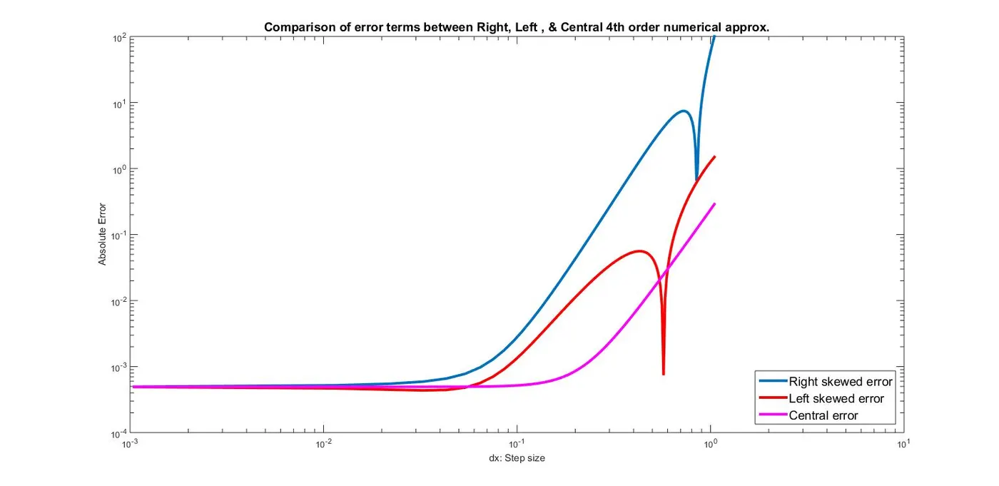
Observations:

• In this case, it's observed that the central difference scheme (CDS) has the least absolute error as step size (dx) increases as compared to the skewed schemes (RSD & LSD).
• The reason for the CDS to have the least error could be due to the fact in symmetry of the nodes chosen to approximate a function at a particular point.

3.b) Describe why a skewed scheme is useful? What can a skewed scheme do that a CD scheme cannot do?

• Skewed scheme is especially useful if approximation by difference is to be performed at the boundary, which is a norm in CFD (eg. at the face of a control volume), and with CDS it is possible only if we make an assumption about the point beneath the boundary (as this point does not exist) which may very well deviate from the physical phenomenon of the problem at hand.