Week 3 - Taylor table method and Matlab code
AIM: -
TO DERIVE THE FOURTH ORDER APPROXIMATION OF A SECOND ORDER DERIVATIVE FUNCTION FOR THE THREE DIFFERENT SCHEMES (CENTRAL DIFFERENCE SCHEME, SKEWED RIGHT&LEFT SIDED DIFFERENCE SCHEME)
TO FIND: -
- CENTRAL DIFFERENCE
- SKEWED RIGHT-SIDED DIFFERENCE
- SKEWEWD LEFT-SIDED DIFFERENCE
ANALYITCAL FUNCTION: -
`e^x*cos(x)`
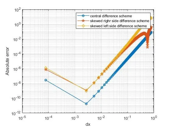
EVALUTE THE ABOVE ANALYTICAL FUNCTION & COMPARE IT WITH THE THREE NUMERICAL APPROXIMATIONS MENTIONED ABOVE.
CODE EXPLANATION: -
- FOR EQUATING THE EQUATIONS WHICH WE CREATED WITH THE TAYLOR TABLE, WE USE ‘’SYMS’’ COMMAND TO SOLVE THE EQUATIONS.
- AFTER SOLVING THE RESPECTIVE EQUATIONS FOR THE THREE DIFFERENT SCHEMES, WE GET THE COEFFICIENTS OF THE VARIABLES USED IN THAT EQUATIONS.
- CREATING A FUNCTION TO EVALUATE THE THREE NUMERICAL FUNCTION WITH THE ANALYTICAL DERIVATIVE.
- CREATING A PROGRAM FOR CALLING THE RESPECTIVE FUNCTION AND ALSO TO CREATE PLOTS WHICH COMPARES THE THREE NUMERICAL APPROXIMATIONS.
THUMB RULE: -
- i) The order of accuracy P= Number of nodes in the stencil N - order of derivative Q + 1 for symmetric/central schemes
- ii) The order of accuracy P= Number of nodes in the stencil N- order of derivative Q for one-sided/skewed schemes
FOR CENTRAL SCHEME = NO: OF: NODES WILL BE 5.
FOR SKEWED SCHEME = NO: OF: NODES WILL BE 6.
CENTRAL DIFFERENCE SCHEME: -
(i-2) (i-1) (i) (i+1) (i+2)
_______________________________________
HERE, WE MARKED THE NODE POINTS WHICH ACTUALLY THE CENTRAL DIFFERNCE LOOK ALIKE
∂^2F/∂X^2 = af(i-2)+bf(i-1)+cf(i)+df(i+1)+ef(i+2)
|
∂^2f/∂x^2 |
f(x) |
f’(x) |
f’’(x) |
f’’’(x) |
(x) |
𝒇𝟱(x) |
|
af(i-2) |
a |
-2a |
4a/2 |
-8a/6 |
16a/24 |
-32a/120 |
|
bf(i-1) |
b |
-b |
b/2 |
-b/6 |
b/24 |
-b/120 |
|
cf(i) |
c |
0 |
0 |
0 |
0 |
0 |
|
df(i+1) |
D |
d |
d/2 |
d/6 |
d/24 |
d/120 |
|
ef(i+2) |
e |
2e |
4e/2 |
8e/6 |
16e/24 |
32a/120 |
|
Co-efficient
|
0
|
0
|
1
|
0
|
0
|
0
|
THE EQUATIONS ARE: -
a+b+c+d+e=0 ❶
-2a-b+d+2e=0 ❷
4a+b+d+4e=2 ❸
-8a-b+d+8e=0 ❹
16a+b+d+16e ❺
SOLVING THE ABOVE EQUATION WE GET CO-EFFICIENTS OF a,b,c,d,e.
a=-1/12, b=4/3, c=-5/2, d=4/3, e=-1/12
By substituting the above co-efficient the central difference will be
∂^2F/∂X^2 = -1*f(i-2)+4*f(i-1)+5*f(i)+4*f(i+1)-1*f(i+2)/12∆x^2.
SKEWED LEFT SIDE DIFFERENCE SCHEME: -
(i-5) (i-4) (i-3) (i-2) (i-1) (i)
______________________________________________
HERE, WE MARKED THE NODE POINTS WHICH ACTUALLY THE SKEWED LEFT SIDE DIFFERNCE LOOK ALIKE
∂^2F/∂X^2 = af(i)+bf(i-1)+cf(i-2)+df(i-3)+ef(i-4)+gf(i-5)
|
∂^2f/∂x^2 |
f(x) |
f’(x) |
f’’(x) |
f’’’(x) |
(x) |
𝒇𝟱(x) |
|
af(i) |
a |
0 |
0 |
0 |
0 |
0 |
|
bf(i-1) |
b |
-b |
b/2 |
-b/6 |
b/24 |
-b/120 |
|
cf(i-2) |
c |
-2c |
4c/2 |
-8c/6 |
16c/24 |
-32c/120 |
|
df(i-3) |
d |
-3d |
9d/2 |
-27d/6 |
81d/24 |
-243d/120 |
|
ef(i-4) |
e |
-4e |
16e/2 |
-64e/6 |
256e/24 |
-1024e/120 |
|
gf(i-5) |
g |
-5g |
25g/2 |
-125g/6 |
625g/24 |
-3125g/120 |
|
Co-efficient
|
0
|
0
|
1
|
0
|
0
|
0
|
THE EQUATIONS ARE: -
a+b+c+d+e+g=0 ❶
-b-2c-3d-4e-5g =0 ❷
b+4c+9d+16e+25g =2 ❸
-b-8c-27d-64e-125g =0 ❹
b+16c+81d+256e+625g=0 ❺
-b-32c-243d-1024e-3125g=0 ❻
SOLVING THE ABOVE EQUATION WE GET CO-EFFICIENTS OF a,b,c,d,e,g.
a=15/4, b=-77/6, c=107/6, d=-13, e=61/12,g=-5/6
By substituting the above co-efficient the skewed left side difference will be
∂^2F/∂X^2 = 45*f(i)-154*f(i-1)+214*f(i-2)-156*f(i-3)+61*f(i-4)-10*f(i-5)/12∆x^2.
SKEWED RIGHT SIDE DIFFERENCE: -
(i) (i+1) (i+2) (i+3) (i+4) (i+5)
_______________________________________________
HERE, WE MARKED THE NODE POINTS WHICH ACTUALLY THE SKEWED RIGHT SIDE DIFFERNCE LOOK ALIKE
∂^2F/∂X^2 = af(i)+bf(i+2)+cf(i+3)+df(i+4)+ef(i+5)+gf(i+6)
|
∂^2f/∂x^2 |
f(x) |
f’(x) |
f’’(x) |
f’’’(x) |
(x) |
𝒇𝟱(x) |
|
af(i) |
a |
0 |
0 |
0 |
0 |
0 |
|
bf(i+1) |
b |
b |
b/2 |
b/6 |
b/24 |
b/120 |
|
cf(i+2) |
C |
2c |
4c/2 |
8c/6 |
16c/24 |
32c/120 |
|
df(i+3) |
d |
3d |
9d/2 |
27d/6 |
81d/24 |
243d/120 |
|
ef(i+4) |
e |
4e |
16e/2 |
64e/6 |
256e/24 |
1024e/120 |
|
gf(i+5) |
g |
5g |
25g/2 |
125g/6 |
625g/24 |
3125g/120 |
|
Co-efficient
|
0
|
0
|
1
|
0
|
0
|
0
|
THE EQUATIONS ARE: -
a+b+c+d+e+g=0 ❶
b+2c+3d+4e+5g =0 ❷
b+4c+9d+16e+25g =2 ❸
b+8c+27d+64e+125g =0 ❹
b+16c+81d+256e+625g=0 ❺
b+32c+243d+1024e+3125g=0 ❻
SOLVING THE ABOVE EQUATION WE GET CO-EFFICIENTS OF a,b,c,d,e,g.
a=15/4, b=77/6, c=107/6, d=13, e=61/12,g=5/6
By substituting the above co-efficient the right side difference will be
∂^2F/∂X^2 = 45*f(i)-154*f(i-1)+214*f(i-2)-156*f(i-3)+61*f(i-4)-10*f(i-5)/12∆x^2.
THESE ABOVE VALUES ARE THE 2ND ORDER AND 4TH ORDER APPROXIMATION.
PROGRAM FOR CENTRAL DIFFERENCE: -
clear all
close all
clc
%inputs for solving central difference scheme
syms a b c d e
eqn_1=a+b+c+d+e==0;
eqn_2=-2*a-b+d+2*e==0;
eqn_3=4*a+b+d+4*e==2;
eqn_4=-8*a-b+d+8*e==0;
eqn_5=16*a+b+d+16*e==0;
eqn=[eqn_1 eqn_2 eqn_3 eqn_4 eqn_5];
S=solve(eqn);
coef_a=S.a;
coef_b=S.b;
coef_c=S.c;
coef_d=S.d;
coef_e=S.e;
PROGRAM FOR SKEWED RIGHT SIDE DIFFERENCE: -
clear all
close all
clc
%input solving skewed right side difference scheme
syms a b c d e g
eqn_1= a+b+c+d+e==0;
eqn_3= b+4*c+9*d+16*e+25*g==2;
eqn_2= b+2*c+3*d+4*e+5*g==0;
eqn_4= b+8*c+27*d+64*e+125*g==0;
eqn_5= b+16*c+81*d+256*e+625*g==0;
eqn_6= b+32*c+243*d+1024*e+3125*g==0;
eqn=[eqn_1 eqn_2 eqn_3 eqn_4 eqn_5 eqn_6];
S=solve(eqn);
coef_a=S.a;
coef_b=S.b;
coef_c=S.c;
coef_d=S.d;
coef_e=S.e;
coef_g=S.g;
PROGRAM FOR SKEWED LEFT SIDE DIFFERENCE: -
clear all
close all
clc
%solving skewed left side difference scheme
syms a b c d e g
eqn_1= a+b+c+d+e+g==0;
eqn_2=-b-2*c-3*d-4*e-5*g==0;
eqn_4=-b-8*c-27*d-64*e-125*g==0;
eqn_3=b+4*c+9*d+16*e+25*g==2;
eqn_5=b+16*c+81*d+256*e+625*g==0;
eqn_6=-b-32*c-243*d-1024*e-3125*g==0;
eqn=[eqn_1 eqn_2 eqn_3 eqn_4 eqn_5 eqn_6];
S=solve(eqn);
coef_a=S.a;
coef_b=S.b;
coef_c=S.c;
coef_d=S.d;
coef_e=S.e;
coef_g=S.g;
FUNCTION PROGRAM: -
function[central_diff,skewed_right_diff,skewed_left_diff,central_error,skewed_left_error,skewed_right_error]=taylor_table_scheme(x,dx,analytical_derivative)
%numerical derivat0ive
central_diff=((-exp_x(x-2.*dx))+(16*exp_x(x-dx))-(30*exp_x(x))+(16*exp_x(x+dx))-(exp_x(x+2.*dx)))./(12*(dx.^2));
skewed_right_diff=((45*exp_x(x))-(154*exp_x(x+dx))+(214*exp_x(x+2.*dx))-(156*exp_x(x+3.*dx))+(61*exp_x(x+4.*dx))-(10*exp_x(x+5.*dx)))./(12*(dx.^2));
skewed_left_diff=((45*exp_x(x))-(154*exp_x(x-dx))+(214*exp_x(x-2.*dx))-(156*exp_x(x-3.*dx))+(61*exp_x(x-4.*dx))-(10*exp_x(x-5.*dx)))./(12*(dx.^2));
%error
central_error= abs(central_diff-analytical_derivative);
skewed_left_error=abs(skewed_left_diff-analytical_derivative);
skewed_right_error=abs(skewed_right_diff-analytical_derivative);
end
function out= exp_x(x,~)
out=(exp(x))*(cos(x));
end
MAIN PROGRAM: -
clear all
close all
clc
% inputs
%analytical_function
x=pi/3;
dx=linspace(pi/4,pi/40000,300);
analytical_derivative=-2*(exp(x))*(sin(x));
% calling functions
for i=1:length(dx)
[central_diff(i),skewed_right_diff(i),skewed_left_diff(i),central_error(i),skewed_right_error(i),skewed_left_error(i)]=taylor_table_scheme(x,dx(i),analytical_derivative);
end
%plotting graphs
loglog(dx,central_error,'linewidth',1,'marker','hexagram')
hold on
loglog(dx,skewed_right_error,'linewidth',1,'marker','pentagram')
hold on
loglog(dx,skewed_left_error,'linewidth',1,'marker','diamond')
hold on
xlabel('dx')
ylabel('Absolute error')legend('central difference scheme','skewed right side difference scheme','skewed left side difference scheme')
grid on
WHY SKEWED SCHEME IS USEFUL AND WHAT CAN A SKEWED SCHEME DO THAT A CD SCHEME CAN’T?
Apparently skewed schemes can be used when direction of flow of a particular entity is known i.e. for example if heat flows over plate from left to right and Skewed right sided scheme is used the solution obtain would contain higher accuracy when compared to CDS.
OUTPUT: -