Week 3 - Solving second order ODEs

Objective:

To write a python program that simulates the motion between 0-20 sec, for angular displacement=0, angular velocity=3 rad/sec at time t=0.

ODE for a motion of a  pendulum with damping

where

b= damping coefficient(kg/s)

l= length of pendulum (m)

m= mass of pendulum(kg)

g= acceleration due to gravity(m/s2)

b=0.05kg/s

l=1m

m=1g

g=9.81m/s^2

Reduction of Order

In order to solve the equation of pendulum using Python first, we should convert second order ode to first order ode

y"+(b/m)y'+(g/l)sin(y)=0                        1

 assume

             y=y1

             y1'=y2

             y1"=y2'

Then we get the following first order ode

y2'=-(b/m)y2-(g/l)sin(y1)                          2

y1'= y2                                                            3

Procedure:

1. "numpy" library function is used to perform array operations in python. In this program, numpy is used to define time steps for integration.
2. "scipy" module is used to perform ode integration for solving the equation of pendulum with damping.
3. "mathplotlib" is used for plotting purposes and "math" is used to perform mathematical operations like sin cos function and so on.
4. Inputs(length of the pendulum, mass of the bob, Damping coefficient, gravity), initial conditions(angular velocity and displacement at time = 0s), and time steps are defined for solving governing equations.
5. "odeint" command is used for performing ODE integration, In order to integrate the equation, first a function(model) should be defined.
6. Syntax for odeint function "scipy.integrate.odeint(func, y0, t, args=())"
7. The function model should contain time steps, initial conditions, and arguments(b,g,L,m) as an input and the function returns the velocity and displacements of the pendulum as an output.

# Defining Function
def model(theta,t,b,g,l,m):
	theta1=theta[0]
	theta2=theta[1]
	dtheta1_dt=theta2
	dtheta2_dt=((-b/m)*theta2)-((g/l)*math.sin(theta1))
	theta=[dtheta1_dt,dtheta2_dt]
	return theta

 This function returns the dtheta1 and dheta2 as the output. The values b,g,l,m can be changed to have different outputs. 

        8. To convert the polar form(theta) to cartesian form(X-Y) following equations are used

     X= L* Sin(theta)

     Y=-L*cos(theta)

      L is the length of the pendulum

       9. For loop is used to find the x y values for all the values of theta.

       10. For animating the motion of the pendulum first the images for all theta values named "number.gif" are collected and saved and those figures are manipulated to appear as moving images.  

Python Program:

import numpy as np 
from scipy.integrate import odeint 
import matplotlib.pyplot as plt 
import math 

# Defining Function
def model(theta,t,b,g,l,m):
	theta1=theta[0]
	theta2=theta[1]
	dtheta1_dt=theta2
	dtheta2_dt=((-b/m)*theta2)-((g/l)*math.sin(theta1))
	theta=[dtheta1_dt,dtheta2_dt]
	return theta


# Inputs
b=0.05
g=9.81
l=1
m=1

# Number of points
n=300

# Initial condition
theta0=[math.radians(0),3]

# Time integration
t=np.linspace(0,20,n)

# Integration
theta=odeint(model,theta0,t,args =(b,g,l,m))
# Plot velocity and displacement with respect to time
plt.plot(t,theta[:,0],'b-')
plt.plot(t,theta[:,1],'r--')
plt.xlabel('Plot')
plt.ylabel('time')
plt.legend(['Displacement','Velocity'])
plt.grid()
plt.show()

'''
b=0.1
g=9.81
l=1
m=1
theta=odeint(model,theta0,t,args =(b,g,l,m))
# Plot velocity and displacement with respect to time
plt.plot(t,theta[:,0],'g-')
plt.plot(t,theta[:,1],'y--')
plt.xlabel('Plot')
plt.ylabel('time')
plt.legend(['Displacement','Velocity'])
plt.grid()
'''


# Locating ball position
x=[]
y=[]
for i in range (0,n):
	x.append(l*math.sin(theta[i,0]))
	y.append(l*-math.cos(theta[i,0]))
	
# axis 
x0=0
y0=0
ct=1

# Animation of motion of the pendulum 

for j in range (0,n):
	filename=str(ct)+'.png'
	ct=ct+1
	plt.figure()
	plt.xlim([-1.5,1.5])
	plt.ylim([-1.5,1])
	plt.plot([-0.5,0.5],[0,0],'blue',linewidth=5)
	plt.plot(x[j],y[j],'o',markersize=20)
	plt.plot([x0,x[j]],[y0,y[j]],'black')
	plt.savefig(filename)

Output:

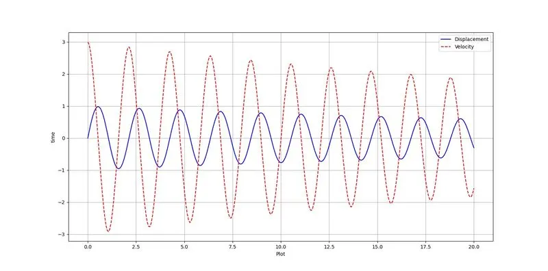
From the graph, it can be seen that at time=0 the angular velocity is 3rad/sec and displacement is 0. The velocity behaves as a cos curve and displacement behaves as as sin curve form. The velocity and displacement gradually decrease with time steps. The decrease in velocity is due to damping.

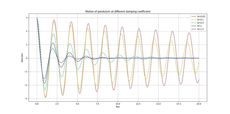
From the graph, it can be inferred that with an increase in damping the velocity of the pendulum is brought to zero at a faster rate.

Error Faced

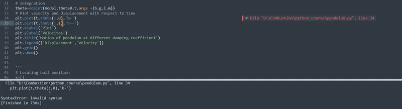
The use of "()" while plotting is the major error and it is rectified by using [] bracket.

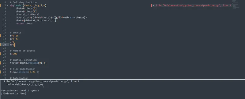
The error is not using : for defining a function (syntax error). The problem is solved by using : command after defining a function.

Conclusion:

• The second-order ode is solved in Python by using odeint command.
• The velocity of the pendulum decreases at a faster rate with an increase in the damping coefficient.

Video Link for Animation

https://youtu.be/OsxnqVHIBy0