Week 3 - Solving second order ODEs

OBJECTIVE: Develop a python code to simulate the Motion of the Pendulum.

PROBLEM STATEMENT:

• Plotting graphs for different angles of displacements that gives corresponding different positions of a pendulum with the help of python code.
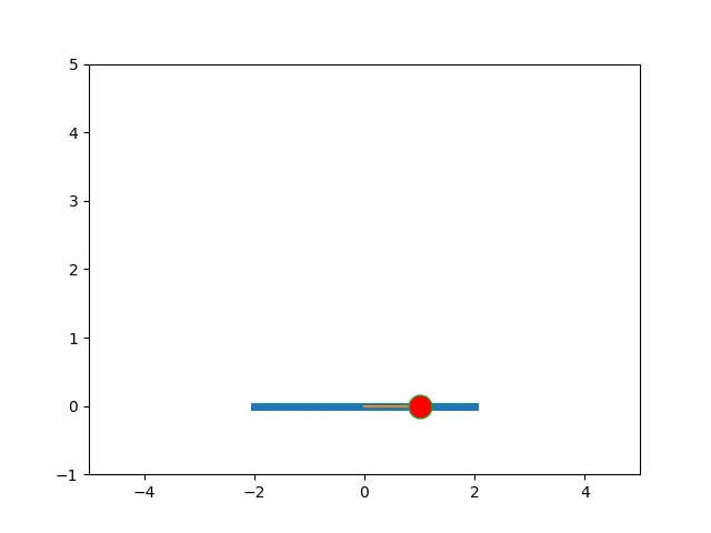
• Creating an animation from the generated plots to display the motion of the simple pendulum.
• Also, plotting the graph which displays the profile of displacement and velocity wrt time.

SOLUTION PROCEDURE:

• At first, knowing the required input parameters involved in the motion of pendulums such as damping coefficient (b) & length of the pendulum (L) and mass of the ball (m), and acceleration due to gravity (g).
• After that, breaking the given second ordinary differential equation into two first-order differential equations.
• 
• Eq 1 and Eq2 represent two sets of first-order differential equations.
• Using ODEINT command to solve the above set of differential equations.
• We are using the modules like {import math} for arithmetic operations required for this objective and also {matplotlib. pyplot as plt} for plotting required graphs and script module for solving the ordinary differential equations and NumPy module to create time array (i.e., time steps for integration).
• Last, converting the generated plots to one gif file using image magick represents the pendulum's motion.

• CODE (with explanation):

  import math
  import matplotlib.pyplot as plt 
  import numpy as np 
  from scipy.integrate import odeint
  
  # Defining a function D which represents ODE systems.
  def D(theta,t,b,g,l,m):
  	theta1=theta[0]     
  	theta2=theta [1]
  	# TWO ORDINARY DIFFERENTIAL EQUATIONS.
  	dtheta1_dt=theta2                                    # First ODE which gives the values of displacement.
  	dtheta2_dt=(-b/m)*(theta2)-(g/L)*(math.sin(theta1))  # Second ODE which gives the values of velocity.
  	dtheta_dt=[dtheta1_dt,dtheta2_dt]                    # Put the above two ODE's into Single ODE i.e dtheta_dt.
  	return(dtheta_dt)                                    # Returning the function.
  
  b=0.05  # DAMPING COEFFICIENT
  g=9.81  # ACCERELATION DUE TO GRAVITY (m/s^2)
  L=1     # LENGTH OF THE STRING (m)
  m=1     # MASS OF THE BALL  (Kg)
  
  # Using the command np.linspace to create a time array which extract 150 values between 0 to 10.
   # We are integrating the above set of differential equations from time ( 0 seconds to 10 seconds).In between we are creating 150 time steps.
  t=np.linspace(0,10,150)
  
  theta_0=[math.pi/2,0]
   # Providing the initial conditions for the two ODE's & ( math.pi/2 is for theta1 i.e displacement and 0 is for theta2 i.e velocity)
   # Solving the above set of differential equations (i.e dtheta_dt) using odeint command.
   # odeint is a command in scipy module.
  theta=odeint(D,theta_0,t,args=(b,g,L,m))
  
  # plotting the above obtained results wrt to time.
  
  plt.figure(1)
  plt.plot (t,theta[:,0],'b--')  # This plot represents the values of displacements.  
  plt.plot(t,theta[:,1],'r--')   # This plot represents the values of velocities.
  plt.ylabel('plot')             # Labelling the X-axis.
  plt.xlabel('time')             # Labelling the Y-axis.
  plt.show()
  
  ct=1
  
  T=theta[:,0]    # Represents displacements values.
  print(T)
  
   # using for loop to create individual plots and combining all the plots to create a animation(.gif file) using image magick
  
  for i in T:
  	x0=0
  	y0=0
  	x1=L*math.sin(i)
  	y1=-L*math.cos(i)
  	print(x1)
  	print(y1)
  	plt.figure(ct)
  	file_name=str(ct)+'.png'
  	plt.plot([-2,2],[0,0],linewidth=5)
  	plt.plot([x0,x1],[y0,y1])
  	plt.plot(x1,y1,marker='o',markersize=15,markerfacecolor='red')
  	plt.xlim(-5,5)
  	plt.ylim(-1,5)
  	plt.savefig(file_name)
  	ct=ct+1
  
  
  
  
  
  
  
  
  
  
  
  
  	

  RESULTS AND DISCUSSIONS:

  Plot (Profiles of displacement & Velocity Vs. Time):

  The blue color curve represents the variation of displacement wrt to time.

  The red color curve represents the variation of velocity wrt to time.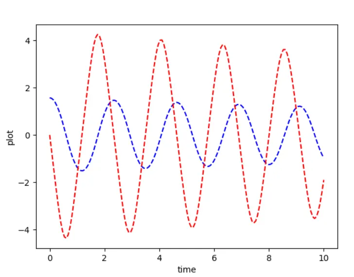
• 

• GIF FILE:

  The gif file which represents the motion of the pendulum:

• 

• YOUTUBE LINK OF THE ANIMATION: https://youtu.be/hV9vki77b0Q