Week 3 - Solving second order ODEs

AIM : to solve ode for the pendulum equations.

theory: a pendulum is a divice which is used in clock it consists of string of length'l' and ball of mass 'm' and gravity at the end at t= 0 it has angular displacement is zero and angular velocity is 3 rad/sec as the pendulum starts moving is makes an angle theta in x axis = l*sin(theta) and y =- l*cos(theta) y this we will able to find out the angular displacement and angular velocity at time range of 0 to 20.

function [dtheta_dt] = ode_difffunc(t,theta,l,m,b,g)

theta1 = theta(1)
theta2 = theta(2)
dtheta1_dt = theta2
dtheta2_dt = -(b/m)*theta2-(g/l)*sin(theta1)
dtheta_dt = [dtheta1_dt ; dtheta2_dt]
end

% inputs
 l = 1 ; % length of a pendulum in mtrs
 m = 1 ; % mass  of a ball in kg
 b = 0.05 ; % damping cofficent
 g = 9.81 ; % gravity in m/s^2
 
 % intial data 
 
 % at time t = 0, angular disp = 0 , angular velocity = 3
 
 theta_0 = [0;3];
 
 t_span = linspace(0,20,500);
 
 % solve
  [t, results] = ode45(@(t,theta)ode_difffunc(t,theta,l,m,b,g),t_span,theta_0);
  
  % plotting
  figure(1)
  plot(t,results(:,1))
  hold on 
  plot(t,results(:,2))
  xlabel('tme in sec')
  ylabel('plot')
  legend('angular displacement','angular velocity')
  title('harmonic motion of pendulum')
  
  ct = 1;
  T = results(:,1);
  for i = 1:length(T)
      X = T(i);
      x0 =0
      y0 =0
      
      x1 =l*sin(X)
      y1 =-l*cos(X)
      
      %plotting(2)
 figure(2)
 plot([-1 1], [0 0],'linewidth',3)
 hold on
 plot([x0 x1], [y0 y1], 'linewidth',3)
 hold on
 plot(x1,y1,'o','markersize',20,'markerfacecolor','b')
 axis([-2 2 -2 2])
 pause(0.03)
 hold off
 ct = ct+1;
 M(ct) = getframe(gcf)
  end
  movie(M)
  videofile = VideoWriter('odinarry_de.avi','uncompressed avi')
  open(videofile)
  writeVideo(videofile,M)
  close(videofile)
  

explanation:

1st we provide the inputs

l = 1; length of a pendulum in mtrs
m = 1 ; mass of a ball in kg
b = 0.05 ; damping cofficent is a property of material wheater is bounce back or return energy to system.
g = 9.81 ; gravity in m/s^2

intial data t =0 the angular displacement 0 and angular velocity is 3rad/s;

theta_0 = [0;3]; at theta =0 ,angular disp = 0 angular vel. =3;

t_span = linspace(0,20,500); is the travel time of pendulum;

% solve
[t, results] = ode45(@(t,theta)ode_difffunc(t,theta,l,m,b,g),t_span,theta_0);is used to get the results at given we used this command ode45 is range kutta 4th order w.r.t time and theta ode_difffunc is function .

% plotting
figure(1)
plot(t,results(:,1)) by using plot command against time and results(:,1) columum 1
hold on
plot(t,results(:,2)) by using plot command against time and results(:,1) columum 2
xlabel('tme in sec') metioninig xaxis with time using xlabel
ylabel('plot')mentioning yaxis with plot using ylabel
legend('angular displacement','angular velocity') legemd command to diffrentiate between the curve
title('harmonic motion of pendulum') for providing title

T = results(:,1);
for i = 1:length(T) by using for loop 1 to results of1st columum

x0 =0 providing intial values at x
y0 =0 providing intial values at y

x1 =l*sin(X) final values at x1

y1 =-l*cos(X)final values at x1

plot([-1 1], [0 0],'linewidth',3)
hold on
plot([x0 x1], [y0 y1], 'linewidth',3) by providing plot commond at different point of x0 x1 and x1 y1 to get a pendulum
hold on
plot(x1,y1,'o','markersize',20,'markerfacecolor','b') markersize for making a ball of size 2o
axis([-2 2 -2 2]) the axis of revolution at [-2 2 -2 2]
at last by movie command we will create a video of pendulum.

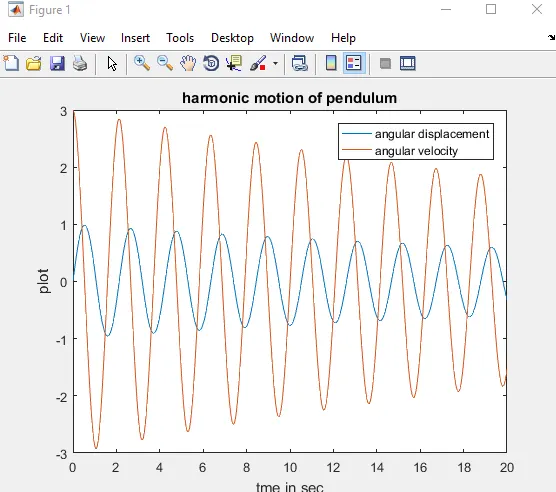
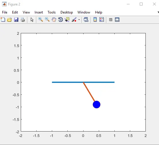
conslusion:perfectly exciution of the curve and motion of pendulum.